Shiva Retrospective Analysis
Alessandro Guida
European Institute of Oncology, MilanGiorgio Melloni
Harvard Medical School, Bostonlibrary(readxl)
library(tibble)
library(DT)
library(purrr)
library(magrittr)
library(dplyr)
library(PrecisionTrialDrawer)
library(ggplot2)
library(parallel)
library(RColorBrewer)
library(VariantAnnotation)
library(org.Hs.eg.db) # GENOME wide annotation for HUman based on Entrez Gene identifiers.
#R helper function library
source("helper_functions.R")
# Define Plot color schema
MYPALETTE <- colorRampPalette(rev(brewer.pal(11, "Spectral")), space="Lab")
set.seed(5)INTRODUCTION
ABOUT the SHIVA trial
The Shiva trial is a proof of concept randomized trial based on targeted therapy using molecular characterization. The trial was aiming at compare convertional therapy with a genomic-driven therapy approach. However the results did not find any difference in progression-free survival (PFS) between the treatment arms. The goal of this retrospective analysis is to verify that the R package PrecisionTrialDrawer (here-hence refered as PTD) can be applied for predicting population allocation in a genomic-driven clinical trial design using alterations from the TCGA repositories.
Clinical trial characteristics
The following information were collected from https://clinicaltrials.gov/show/NCT01771458
- Phase II trial;
- Compare two treatment strategies from patients with refractory cancer;
- Tumor biopsy leads to molecular characterization (mutations, amplifications, hormone receptor status). If molecular abnormality is identified, patients are randomied between
- Targeted therapy based on molecular profiling;
- Conventional therapy based on investigator’s choice.
- Intervention
- Drug: Targeted therapy based on molecular profiling : Imatinib
- Procedure: Tumor biopsy
- Drug: Standard Chemotherapy
- Drug: Targeted therapy based on molecular profiling : Everolimus
- Drug: Targeted therapy based on molecular profiling : Vemurafenib
- Drug: Targeted therapy based on molecular profiling : Sorafenib
- Drug: Targeted therapy based on molecular profiling : Erlotinib
- Drug: Targeted therapy based on molecular profiling : Lapatinib + Trastuzumab
- Drug: Targeted therapy based on molecular profiling : Dasatinib
- Drug: Targeted therapy based on molecular profiling : Tamoxifen (or letrozole if contra-indication)
- Drug: Targeted therapy based on molecular profiling : Abiraterone
- Primary Outcome Measures:
- Patient’s progression free survival (according RECIST 1.1) of targeted therapy based on molecular profiling versus conventional chemotherapy.
- Tumor evaluation according to RECIST 1.1 criteria (every 2 months)
- Secondary Outcome Measures:
- Overall response rate (ORR)
- Tumor evaluation according to RECIST 1.1 criteria (every 2 months)
- Overall Survival (OS)
- Patient’s progression free survival (according RECIST 1.1) of targeted therapy based on molecular profiling versus conventional chemotherapy after cross-over.
- more at https://clinicaltrials.gov/show/NCT01771458
Technical considerations
Sequencer used: ION Torrent PGM.
NGS targeted sequencing panels used:
- Ion Ampliseq cancer panel V1
- Ion Ampliseq cancer panel V2
CNA detection
Selected gene copy number alterations (amplification or deletion) were assessed using Cytoscan HD according the manufacturer protocol (Affymetrix®).
Short Results Summury
At the time of the publication on lancet (july 11 2014), the authors have screened 496 patients from different tumor types. 203 had no targetable molecular alteration and 293 (59.1%) patients were enrolled in the study.
- Around the cutoff time, jan 20 2015, 195 (26%) patients had been randomly assigned
- 99 in experimental group;
- 96 in control group;
Retrospective analysis
The objective of this retrospective analysis is to verify that the TCGA population can be used to predict the population allocation in a real clinical trial design. We will use the R package PTD to model the design of the SHIVA trial. Then, we will import the raw data from the population recruited at the time of the trail (kindly provided by the authors of the SHIVA trial), download the TCGA data and adjust the population to match the tumor type distribution recruited in SHIVA. Lastly, using PTD we will investigate on the performance of the two population. More specifically we will compare the:
- ANALYSIS 1) % of patients found to have an alteration that could be allocated to the targeted therapy group;
- ANALYSIS 2) Gene alteration frequency;
- ANALYSIS 3) Patient allocation;
- ANALYSIS 4) Power analysis of the study.
PRE-PROCESSING - prepare the Input
We need to prepare the following inputs
- SHIVA clinical trail design: design of the panel
- SHIVA population
- TCGA population
1. SHIVA clinical trail design: design of the panel
The first objective is to model the original design of the SHIVA trial.
Create a CancerPanel object based on the design suggested in the paper of the SHIVA trial, Supplementary Table S3. In the SHIVA trial, molecular alteration were groups in three 3 molecular pathways:
- Hormone receptor pathway (ER, PR and AR overexpression)
- PI3K/AKT/mTor Pathway
- RAK/MEK pathway
In case of multiple alteration, the allocation was discussed in the Molecular Biology Board (MBB) and alteration were discussed using the following criteria:
- Any mutation, amplification or deletion was considered of a higher impact than hormone receptor expression.
- In case of several mutation/amplification/deletion, the MBB consider the direct targets of MTA as of higher priority for treatment decision. Well known mutations were considered high in the list.
- If expression of both AR and ER/PR in same patient, the hormone receptor with higher expression level was taken in account.
AR (Androgen receptor), ER (Estrogen receptor) and PR (Progesterone receptor) were quantified with Immunohistochemistry. Unfortunately we were not able to simulate IHC values with the TCGA, and this part of the trial was left out.
#import SHIVA Design
# --------------------------------------------------------------------------------
SHIVA_design <- readxl::read_excel("version_6.0/Supplementary_file/SHIVA_design_v6.1.xlsx"
                                    , sheet = 1
                                    , col_types = c("text", "text", "text", "text", "text", "text"))

#fixing input
SHIVA_design$mutation_specification <- as.character(SHIVA_design$mutation_specification)
SHIVA_design$mutation_specification <- sub("\"\"", "", SHIVA_design$mutation_specification)

#CONVERT AMINOACIT TO FORMAT COMPATIBLE FOR PANEL
for (i in 1:nrow(SHIVA_design)) {

  if (!is.na(SHIVA_design$mutation_specification[i]) &&
     SHIVA_design$mutation_specification[i] != "" &&
     SHIVA_design$mutation_specification[i] != "truncating") {

    #Print modification
    cat("Gene", as.character(SHIVA_design$gene_symbol[i]), ":"
        , SHIVA_design$mutation_specification[i]
        , "-->", convertAA(SHIVA_design$mutation_specification[i])
        , "\n")

    #use the helper function to convert the a.a.
    SHIVA_design$mutation_specification[i] <- convertAA(SHIVA_design$mutation_specification[i])
  }
}
## Gene AKT1 : Glu17Lys --> E17K
## Gene PIK3CA : Glu545Lys --> E545K
## Gene PIK3CA : Glu542Lys --> E542K
## Gene PIK3CA : His1047Arg --> H1047R
## Gene PIK3CA : Thr1025Ala --> T1025A
## Gene PIK3CA : Glu453Lys --> E453K
## Gene PIK3CA : Gln546Lys --> Q546K
## Gene BRAF : Gly469Ala --> G469A
## Gene BRAF : Val600Glu --> V600E
## Gene ERBB2 : Ser792Phe --> S792F
## Gene ERBB2 : Thr862Ala --> T862A
## Gene FLT3 : Met665Thr --> M665T
## Gene KIT : Val852Ile --> V852I
## Gene KIT : Asp572Gly --> D572G
## Gene KIT : Met722Val --> M722V
## Gene KIT : Pro838Ser --> P838S
## Gene PDGFRA : Leu655Trp --> L655W# preview
# --------------------------------------------------------------------------------
datatable_withbuttons(SHIVA_design)2. SHIVA population
The original data collected during the SHIVA trials, were provided to us by the authors as an excel file, one with SNV information as well as aggregated data, one with the CNA profile.
Import raw data
Import in the analysis the raw data. Add a column with the TCGA tumor ID confersion Supplementary_file/SHIVA_conversiontable.xlsx.
# Read in SHIVA raw data
merged_df <- readxl::read_excel("version_6.0/Supplementary_file/SHIVA_authorTable.xlsx"
                                  , sheet = 1
                                  , col_names = TRUE
 #                                , col_types = rep("text", times=24)
                                 )

# Import CNA data for the 496 profiled patients

cna_data <- readxl::read_excel("version_6.0/Supplementary_file/SHIVA_cna_data.xls"
                                , sheet = 1
                                , col_names = TRUE)
Adjust shiva population
The objective in this section is to filter out patients that could create problem in the comparison. Using the SHIVA authors table, we want to keep those patients with:
- Localizations compatible with TCGA, we will remove patients with tumor location without a clear match to the TCGA tumor types.
- remove those patients that do not have NGS or CNA performed. (this will reduce the dataset to only those that are actually with a complete profile).
- find patients with no CNA data (all genes tested for CNA, in case one observation was missing it was marked as “NA”).
- We are no longer including HR in the analysis. So we have removed the filter on expression.
of the remaing now, you can check how many are eligible for randomization and therefore calculate the expected detected fraction.
Select patients with a full data profile (NGS + CNA) on which to run some population inference.
We have not removed those patients that were not randomized for any particular reasons (death, consensus withdrawal, ..) as long as the mutational profile is known.
Finally, we removed patients with TCGA tumor types acyc, sclc, es, because have no CNA data in TCGA population.
The following table shows the patients consituting the SHIVA population for this analysis.
# Patient filtering
# ------------------------------------------------------------------------------
# All patients have CNA data, so we do not include any filter here.
df_full_profile <- merged_df %>%
  # filter by patients that do not have a Complete profile: CNA are OK, no patients filtered there.
  # Filter those patient without a complete NGS profile (for SNV analysis)
  dplyr::filter(!NGS == "Not done") %>%
  # filter those patients with locations incompatible with the TCGA
  dplyr::filter(!TCGA_tumor_ID == "") %>%
  # Remove patients that were not randomized because of problems
  # dplyr::filter(Reason.for.no.randomization == "ERROR")
  # Remove patients with tumor types  acyc, sclc, es, becuase have no CNA data in TCGA population
  dplyr::filter(!TCGA_tumor_ID %in% c("acyc", "sclc", "es"))

# Define tumor type list in the population
# -------------------------------------------------------------------------------
tumor_types <- as.character(unique(df_full_profile$TCGA_tumor_ID))
# calculate weights
tumor_weights <- table(as.character(df_full_profile$TCGA_tumor_ID))
# calculate frequency
tumor_freq <- prop.table(tumor_weights)

# Preview
# --------------------------------------------------------------------------------
datatable_withbuttons(df_full_profile, caption = "Patients with a complete profile")
The population recruited in the trial is composed by differnt types of tumor types (after conversion to TCGA tumor ids). The following barplot shows the number of patient for each tumor type.
data.frame(tumor_weights) %>%
  dplyr::rename(Tumor = Var1, Count = Freq) %>%
  dplyr::mutate(Tumor = factor(Tumor
                               , level = Tumor[order(Count)])) %>%
  ggplot(aes(Tumor, Count)) +
    geom_bar(stat="identity", position=position_dodge() ) +
    ggtitle("Number of patient for each tumor type in the SHIVA population") +
    coord_flip()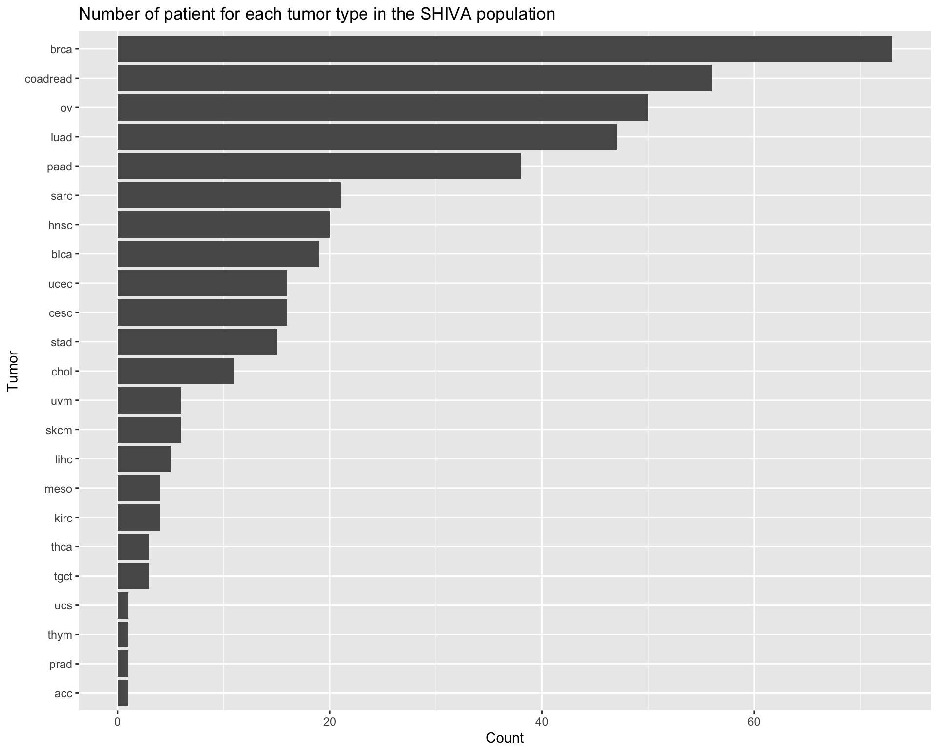
Convert the raw data from the SHIVA study to a PTD population object
In this paragraph we will convert the SHIVA dataset to a format compatible with PTD. Once correctly formatted, it will be imported as a “population background”. Together, with the TCGA data we will have have two population backgrounds, the SHIVA, and the TCGA. We will be able to compare them and investigate whether TCGA data can simulate the SHIVA situation.
Prepare CNA data
For each gene, in each patient, it was reported a CNA status. For a small percentage of cases, the value reported was ambigous (e.g. “amplification, normal, delete_het”).
################################################################################
# CONVERT SHIVA POPULATION TO BE CAMPATIBLE WITH PTD
################################################################################


################################################################################
# PREPARE CNA DATA
# ------------------------------------------------------------------------------
# dataFull Structure
# LIST:
#  $copynumber
#     $data
#        $gene_symbol
#        $CNA
#        $case_id   (sample names with at least one alteration)
#        $tumor_type
#     $Samples
#        $brca  (all screened samples)

# Create Data
# ----------------------
cna_long <- cna_data %>%
  lapply(as.character) %>%
  data.frame(stringsAsFactors=FALSE) %>%
  tidyr::gather("gene_symbol", "CNA", 2:ncol(cna_data)) %>%
  dplyr::select(gene_symbol, CNA, case_id = Patient.ID) %>%
  # Filter by patients.ID we are interested in
  dplyr::filter(case_id %in% df_full_profile$Patient.ID) %>%
  #dplyr::mutate(tumor_type="SHIVA") %>% # add fake tumor name
  dplyr::mutate(case_id=as.character(case_id)) # conver fctr to chr

# preview before correction
cna_long %>%
  dplyr::group_by(CNA) %>%
  dplyr::summarise(counts = n()) %>%
  ggplot(aes(x=reorder(CNA, counts), y=counts)) +
    geom_bar(stat="identity", position=position_dodge()) +
    labs(title="CNA Alterations types (BEFORE correction)") +
    coord_flip()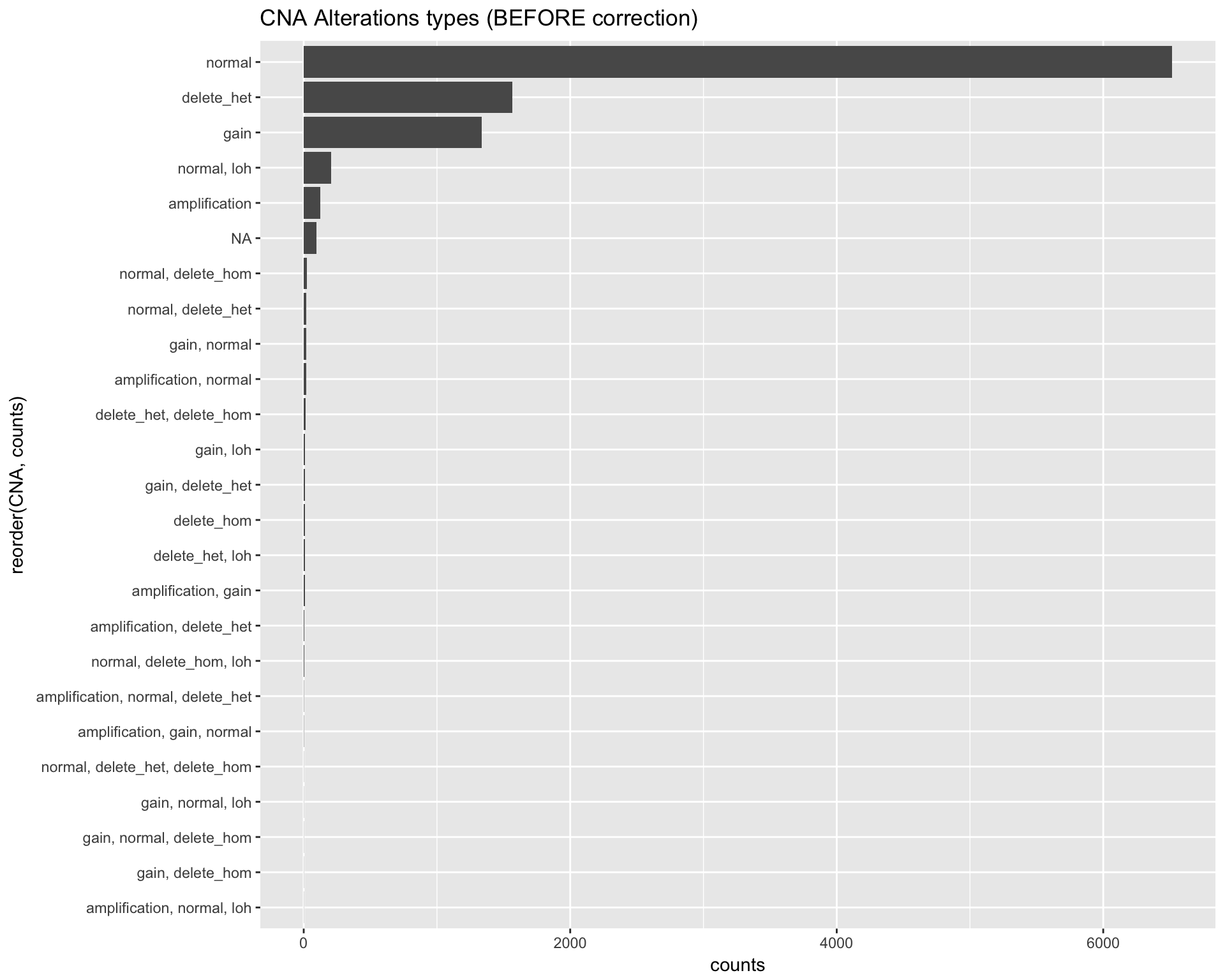
In this paragraph we will perform a correction on the CNA value, by making all the values match one of the following standard states:
- Amplification
- Deletion
- Normal
We considered as deleted, only homologous deletions (as in the Clinical trial).
fixIT <-  function(from, to, target=cna_long$CNA){
  #print(paste("^",from,"$", sep=""))
  gsub(paste("^",from,"$", sep=""), to , target)
}

# fix CNA encoding
# ------------------------------------------------------------------------------
cna_long$CNA <- fixIT("delete_hom",                     "deletion")
cna_long$CNA <- fixIT("normal, delete_het, delete_hom", "deletion")
cna_long$CNA <- fixIT("delete_het, delete_hom",         "deletion")
cna_long$CNA <- fixIT("delete_het, loh",                "deletion")
cna_long$CNA <- fixIT("normal, delete_hom, loh",        "deletion")
cna_long$CNA <- fixIT("normal, delete_hom",             "deletion")

# Convert to normal (ambigous amplifications)
# ------------------------------------------------------------------------------
cna_long$CNA <- fixIT("amplification, normal, delete_het", "normal")
cna_long$CNA <- fixIT("amplification, normal, loh",        "normal")
cna_long$CNA <- fixIT("gain, delete_het",                  "normal")
cna_long$CNA <- fixIT("gain, delete_hom",                  "normal")
cna_long$CNA <- fixIT("gain, normal, delete_hom",          "normal")
cna_long$CNA <- fixIT("normal, delete_het",                "normal")

cna_long$CNA <- fixIT("amplification, delete_het",     "normal")
cna_long$CNA <- fixIT("delete_het",                    "normal")
cna_long$CNA <- fixIT("gain, loh",                     "normal")
cna_long$CNA <- fixIT("gain",                          "normal")
cna_long$CNA <- fixIT("gain, normal, loh",             "normal")
cna_long$CNA <- fixIT("NA",                            "normal")
cna_long$CNA <- fixIT("normal, loh",                   "normal")
cna_long$CNA <- fixIT("gain, normal",                  "normal")

cna_long$CNA <- fixIT("amplification, gain",           "normal")
cna_long$CNA <- fixIT("amplification, gain, normal",   "normal")
cna_long$CNA <- fixIT("amplification, normal",         "normal")

# Get patients list and associated tumor id
# ------------------------------------------------------------------------------
temp <- df_full_profile %>%
  mutate(case_id = as.character(Patient.ID)) %>%
  dplyr::select(tumor_type = TCGA_tumor_ID
                ,  case_id)


# join patients
cna_long <- dplyr::left_join(cna_long, temp, by= "case_id")

# Create Sample
# ----------------------
# get list of tumors
tumor_chr <-  df_full_profile$TCGA_tumor_ID %>%
  unique %>%
  as.character

# prepare funtion to extract sample names for each tumor
sampleXtumor <- function(x, df){
  df %>%
    dplyr::select(Patient.ID, TCGA_tumor_ID) %>%
    dplyr::filter(TCGA_tumor_ID %in% x) %>% .[["Patient.ID"]] %>%
    as.character() %>%
    unique()
}
# Extract samples for each tumors
Samples <- purrr::map(tumor_chr, ~ sampleXtumor(., df=df_full_profile))
names(Samples) <- tumor_chr

# Check if there are problems.
testthat::expect_equal(length(unique(cna_long$case_id)), nrow(df_full_profile))
testthat::expect_equal(length(unlist(Samples)), nrow(df_full_profile))

# Create list element for CNA for the DataFull argument of the panel (panel@DataFull)
# ----------------------
copynumber <- list(  data = data.frame(cna_long)
                   , Samples = Samples)
Preview the CNA dataset after the correction:
copynumber$data %>%
  dplyr::group_by(CNA) %>%
  dplyr::summarise(counts = n()) %>%
  ggplot(aes(x=CNA, y=counts)) +
    geom_bar(stat="identity", position=position_dodge()) +
    labs(title="CNA Alterations types (after correction)") +
    coord_flip()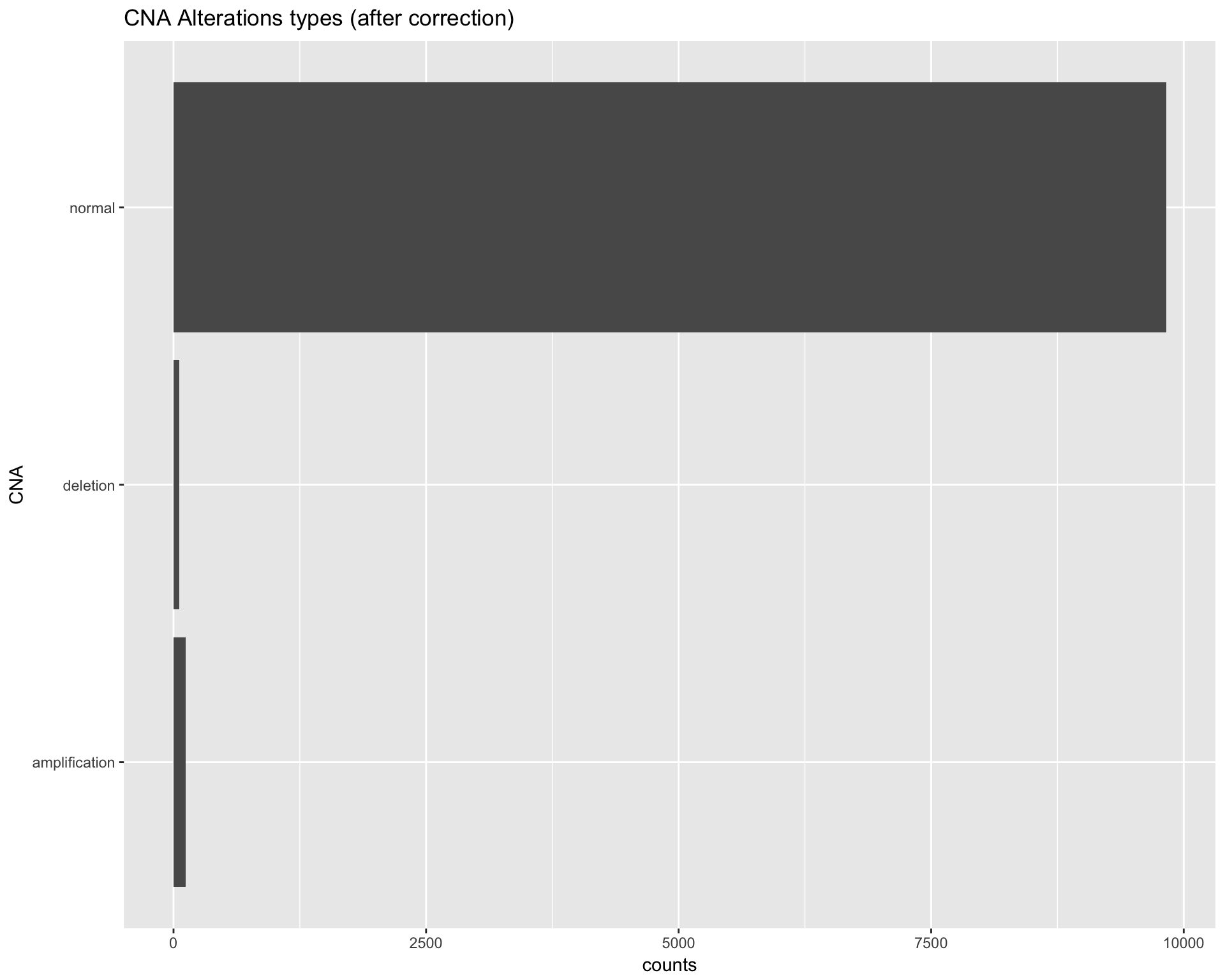
Preview the CNA dataset in a data table.
copynumber$data %>%
  dplyr::group_by(gene_symbol, CNA) %>%
  dplyr::summarise(counts = n()) %>%
  DT::datatable(caption = "Alterations Split by gene")
Preview the Alteration count split by gene:
copynumber$data %>%
  dplyr::filter(CNA %in% c("amplification", "deletion")) %>%
  dplyr::group_by(gene_symbol, CNA) %>%
  dplyr::summarise(counts = n()) %>%
  DT::datatable(caption = "Alterations Split by gene (keep only deletion and amplification terms)")
# Alterations Split by gene (keep only deletion and amplification terms
copynumber$data %>%
dplyr::filter(CNA %in% c("amplification", "deletion")) %>%
dplyr::group_by(gene_symbol, CNA) %>%
dplyr::summarise(counts = n()) %>%
ggplot(aes(x=gene_symbol, y=counts, fill=CNA)) +
geom_bar(stat="identity", position=position_dodge()) +
labs(title="Alterations Split by gene (keep only deletion and amplification terms)") +
coord_flip()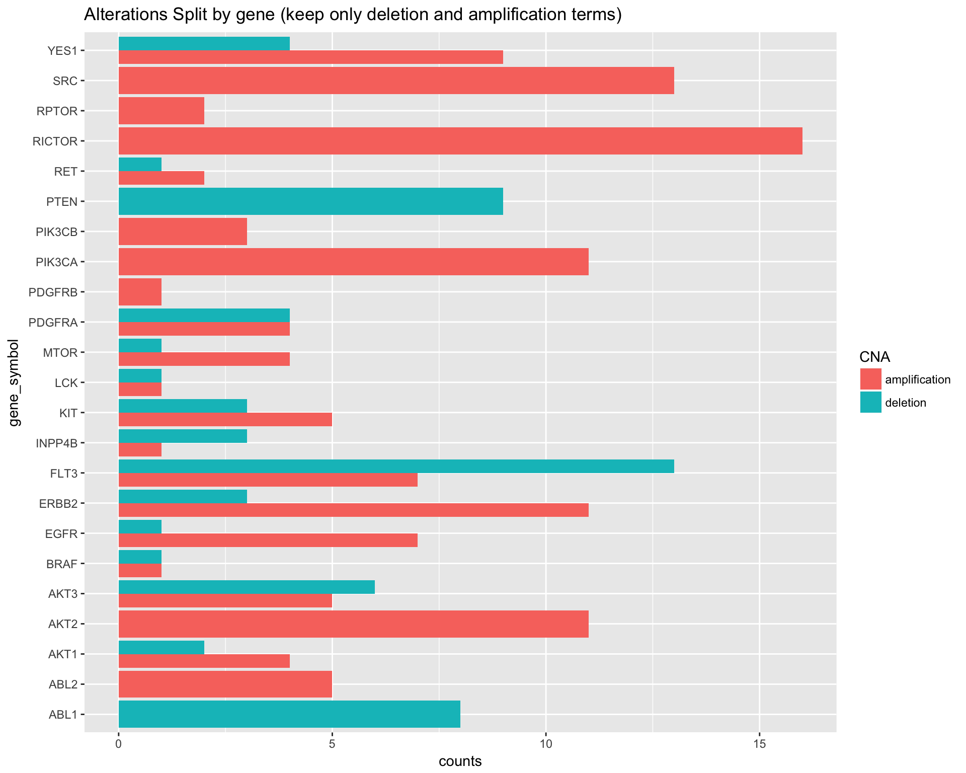
Prepare SNV data
Convert the SNV data into a format compatible with PTD.
Some of the gene names in the raw data were corrected
- RAPTOR <- RPTOR
- PI3KCA <- PIK3CA
- PIK3CB <- PI3KCB
################################################################################
# PREPARE MUTATION DATA
# ------------------------------------------------------------------------------
#   str(panel@dataFull$mutations)

# Convert Gene Name to HGNC standard
# --------------------------------------
wrongGName <- c("RAPTOR","PI3KCA","PIK3CB")
rightGName <- c("RPTOR"  ,"PIK3CA"  ,"PI3KCB")
df_full_profile$gene_symbol <- plyr::mapvalues(df_full_profile$Mutated_genes
                                               , from = wrongGName
                                               , to=rightGName
                                               , warn_missing = FALSE)

# Select fields of interest and start preformatting
#--------------------------------------
mutation_data <- df_full_profile %>%
  dplyr::select(Patient.ID
                , amino_acid_change = pp_old
                , tumor_type = TCGA_tumor_ID
                , gene_symbol
                #, nm = NM_old
                ) %>%
  dplyr::mutate(amino_acid_change = as.character(amino_acid_change)
                , tumor_type = as.character(tumor_type)
                #, nm = as.character(nm)
                )

# Unnesting Genes and the data
###################################################

# split genes and mutations by ";"
# -----------------------------------------------
genes <- strsplit(mutation_data$gene_symbol, ";")
mutations <- strsplit(mutation_data$amino_acid_change, ";")

# Quality check -  remove those patients that have ambiguos SNV annotations
# -----------------------------------------------
gene_lengths <- purrr::map_int(genes, length)
mutations_lengths <- purrr::map_int(mutations, length)

# init patiets to be removed
index_TOBEREMOVED <- c()

# 1. Remove genes that have not the number of mutatiosn
index <- gene_lengths != mutations_lengths
if (any(index)) {

  warning("Problem with imported raw data: the number of alterated genes, does not match the number of SNV alterations. The patient affected by this problem will be removed the analysis\n")

  # show message with ruther details
  message("patients removed:\n", as.character(mutation_data[index, "Patient.ID"]))

  # FIX - REMOVE THEM
  # ~~~~~~~~~~~~~~~~~
  #mutation_data <- mutation_data[-which(index),]
  index_TOBEREMOVED <- index
}
## Warning: Problem with imported raw data: the number of alterated genes, does not match the number of SNV alterations. The patient affected by this problem will be removed the analysis## patients removed:
## c("08-0024", "03-0007", "04-0025", "05-0042", "06-0096", "07-0099", "06-0113", "07-0027", "04-0039")# 2. Remove genes that have one NA in genes or Mutations and
# not a corresponding NA in the other field.
index2 <- is.na(genes) != is.na(mutations)
if (any(index2)) {
warning("Problem with imported raw data: some ambigous annotation in some genes-mutations. Patients affected will be removed\n")
# show message with ruther details
message("patients removed:\n", as.character(mutation_data[index2, "Patient.ID"]))
# FIX - REMOVE THEM
# ~~~~~~~~~~~~~~~~~
#mutation_data <- mutation_data[-which(index2),]
index_TOBEREMOVED <- c(index_TOBEREMOVED, index2)
}## Warning: Problem with imported raw data: some ambigous annotation in some genes-mutations. Patients affected will be removed## patients removed:
## c("07-0098", "01-0222")if(length(index_TOBEREMOVED)>0){
# remove patients that were selected for removal
mutation_data <- mutation_data[-which(index),]
}
# Unnesting genes and alterations
# -----------------------------------------------
unnested_gene <- mutation_data %>% tidyr::separate_rows(gene_symbol, sep = ";")
unnested_pp <- mutation_data %>% tidyr::separate_rows(amino_acid_change, sep = ";")
#merge them back together
unnested_gene$amino_acid_change <- unnested_pp$amino_acid_change
# unnest alterations, second level, split by "|"
unnested_df <- unnested_gene %>%
tidyr::separate_rows(amino_acid_change, sep = "\\|")# %>% unique
# Quality Control
# ----------------------------------------------
if(sum((unnested_df$amino_acid_change) != "", na.rm = TRUE) + sum(is.na(unnested_df$amino_acid_change))
!= purrr::map_int(strsplit(mutation_data$amino_acid_change, ";|\\|"), length) %>% sum()){
stop("unnesting did not work as expected")
}
unnested_df <- unique(unnested_df)
# Adjust AA change
#--------------------------------------
unnested_df$amino_acid_change <- sub("^p." , "" , unnested_df$amino_acid_change)
unnested_df$amino_acid_change <- sub("[" , "" , unnested_df$amino_acid_change, fixed = TRUE)
unnested_df$amino_acid_change <- gsub("Qln" , "Gln" , unnested_df$amino_acid_change, fixed = TRUE)
# conver amminoacid for from long to short
unnested_df$amino_acid_change <- purrr::map_chr(unnested_df$amino_acid_change, hgvs_long_to_short)
# Fix strange simbols
unnested_df <- unnested_df %>%
mutate_cond(amino_acid_change %in% c("NA", "", "XXXX"), amino_acid_change = NA) # custom made conditional mutate
# parse aa position
unnested_df$amino_position <- stringr::str_extract(unnested_df$amino_acid_change , "\\d+")
# 2. Remove genes that have one NA in genes or Mutations and
# not a corresponding NA in the other field.
index2 <- is.na(unnested_df$gene_symbol) != is.na(unnested_df$amino_acid_change)
if (any(index2)) {
warning("Problem with imported raw data: some ambigous annotation in some genes-mutations. Patients affected will be removed\n")
# show message with ruther details
message("patients removed:\n", as.character(unnested_df[index2, "Patient.ID"]))
# FIX - REMOVE THEM
# ~~~~~~~~~~~~~~~~~
unnested_df <- unnested_df[-which(index2),]
}## Warning: Problem with imported raw data: some ambigous annotation in some genes-mutations. Patients affected will be removed## patients removed:
## c("01-0202", "06-0097", "07-0098", "01-0222")# Extract and prepare Sample info
#--------------------------------------
temp_sampledf <- unnested_df %>% dplyr::select(Patient.ID, TCGA_tumor_ID = tumor_type)
tumor_chr <- unique(temp_sampledf$TCGA_tumor_ID)
Samples <- purrr::map( tumor_chr, ~ sampleXtumor(., df= temp_sampledf))
names(Samples) <- tumor_chr
# Subset dataset where there are mutations
#--------------------------------------
# !!!(THIS HAS TO BE DONE AFTER, RETRIEVING THE SAMPLES for the panel structure) !!!!
# otherwise we risk to miss patients that are not included simply becuase they have no alteration
# Load entrez ID
xx <- as.list(org.Hs.egALIAS2EG)
# Remove pathway identifiers that do not map to any entrez gene id
xx <- xx[!is.na(xx)]
unnested_df <- unnested_df %>%
dplyr::filter(!gene_symbol == "") %>% # remove those patients that DO NOT have a gene matched to an alteration
dplyr::mutate(Entrez_gene_ID = sapply(gene_symbol , function(x) as.integer(xx[[x]][1])))
# Very shallow classification of variants
unnested_df$mutation_type <- with( unnested_df ,
ifelse(grepl("Ter$" , amino_acid_change) , "Nonsense_Mutation" ,
ifelse(grepl("fs$" , amino_acid_change) , "Frame_Shift_Ins" ,
ifelse(grepl("del$" , amino_acid_change) , "Frame_Shift_Del" ,
ifelse(grepl("ins" , amino_acid_change) , "Frame_Shift_Ins" ,
"Missense_Mutation"))))
)
# dummy genomic positon as a place holder
unnested_df$genomic_position <- "1:11111:C,G"
#"7:140439656:C,G"
# dummy genetic profile as a place holder
unnested_df$genetic_profile_id <- unnested_df$tumor_type
# change name of Patient.ID column to case_id
#colnames(unnested_df)[colnames(unnested_df)=="Patient.ID"] <- "case_id"
# SOrf df
mutations_df <- unnested_df %>%
dplyr::select(entrez_gene_id= Entrez_gene_ID
, gene_symbol
, case_id = Patient.ID
, mutation_type
, amino_acid_change
, genetic_profile_id
, tumor_type
, amino_position
, genomic_position
) %>%
dplyr::mutate(amino_position = as.integer(amino_position)) %>%
dplyr::mutate(case_id = as.character(case_id))
# Create list element for CNA for the DataFull argument of the panel (panel@DataFull)
# ----------------------
mutations <- list( data = data.frame(mutations_df)
, Samples = Samples)
# PUT THEM TOGETHER
################################################################################
fusion = list(data = NULL
, Samples = NULL
)
expression = list(data = NULL
, Samples = NULL
)
SHIVA_repo <- list(fusions = fusion
, mutations = mutations
, copynumber = copynumber
, expression = expression
)Preview the SNV data to be imported
mutations$data %>%
  dplyr::group_by(gene_symbol) %>%
  dplyr::summarise(count=n()) %>%
  ggplot(aes(x=reorder(gene_symbol, count), y=count)) +
    geom_bar(stat="identity", position=position_dodge()) +
    labs(title="Total SNV (before any filtering) from the SHIVA population") +
    coord_flip()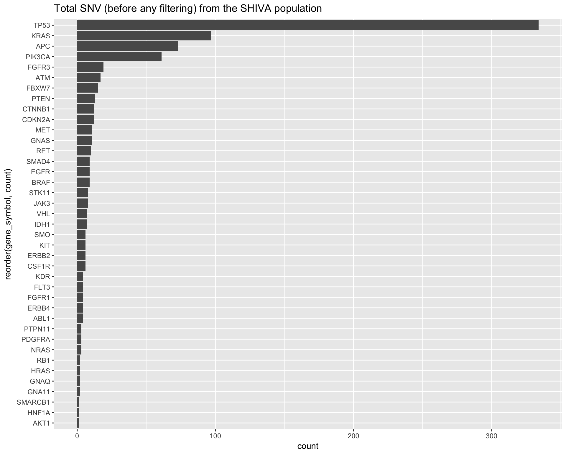
Convert the SHIVA population data into a PTD compatible format
This can be achieved using the build in argument “repo” from the PTD package.
# DESIGN
SHIVA_population <- newCancerPanel(SHIVA_design)
#DOWNLOAD alternative
SHIVA_population <- getAlterations(SHIVA_population
                              , tumor_type = tumor_types
                              , repos = SHIVA_repo
                              )
#SIMULATE
SHIVA_population <- subsetAlterations(SHIVA_population)

#save a backup copy to speed up future analysis
saveRDS(SHIVA_population, file = "version_6.0/Temp/SHIVA_population.rds")
Since we are interested in balancing the TCGA population to make it match with the recruited SHIVA population, we need to estimate how many patients per tumor types will be used.
We can calculate this number “adjusting weight” looking at those patients that have both CNA and SNV data.
Number of patients per tumor type divided by dataset type:
# check pop size from CNA
mya <- purrr::map_int(SHIVA_population@dataFull$copynumber$Samples, length) %>%
  data.frame(count = .) %>%
  tibble::rownames_to_column("tumor_id") %>%
  dplyr::mutate(origin="CNA")

# check pop size from Mutations
myb <- purrr::map_int(SHIVA_population@dataFull$mutations$Samples, length) %>%
  data.frame(count = .) %>%
  tibble::rownames_to_column("tumor_id") %>%
  dplyr::mutate(origin="mutations")

# calculate adjusting weight
# ------------------------------------------------------------------------------
# tumor_weights will be the vector to adjust the TCGA population
tumor_weights <- names(SHIVA_population@dataFull$copynumber$Samples) %>%
  purrr::map(function(tumor_name){

    mut = SHIVA_population@dataFull$mutations$Samples[[tumor_name]]
    cna = SHIVA_population@dataFull$copynumber$Samples[[tumor_name]]

    # find intersection of patients
    output <- length(mut %in% cna)
    names(output) = tumor_name

    return(output)

  }) %>% flatten_int

# check pop size used internally for adjusting TCGA
myc <- tumor_weights %>%
  data.frame(count = .) %>%
  tibble::rownames_to_column("tumor_id") %>%
  dplyr::mutate(origin="new adjusting weight")

# generate a plot
rbind(mya, myb, myc) %>%
  ggplot(aes(tumor_id, count, fill=origin)) +
  geom_bar(stat="identity", position= position_dodge()) +
    coord_flip() +
    ggtitle("number of patients per alteration type from SHIVA.")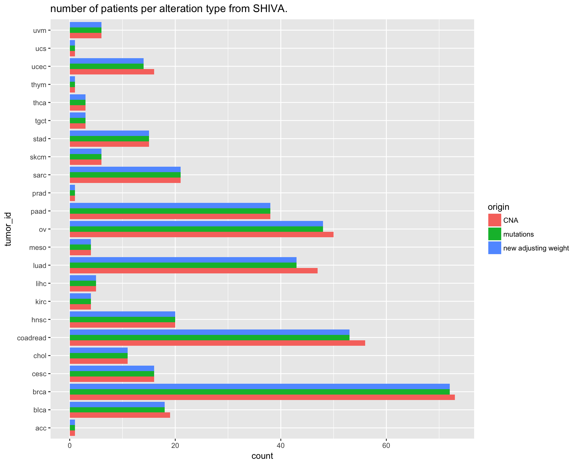
3. TCGA population
Simulate Clinical trial on TCGA population
# DESIGN
TCGA_population <- newCancerPanel(SHIVA_design)
#DOWNLOAD alternative
TCGA_population <- getAlterations(TCGA_population
                              , tumor_type = tumor_types
                              , expr_z_score = 1
                              )
#SUBSET
TCGA_population <- subsetAlterations(TCGA_population)

#save a backup copy to speed up future analysis
saveRDS(TCGA_population, file = "version_6.0/Temp/TCGA_population.rds")
Filter pathogenic mutation
In this section we will apply a filter to remove all the NON pathogenic mutation fetched from cosmic dataset (01-05-2017).
# save the number of entries in the TCGA beofere any filtering
TCGA_original_number <- nrow(unique(TCGA_population@dataFull$mutations$data))

# Clean TCGA popualation running a cosmic filter
cosmic <- readr::read_csv("version_6.0/external_resources/cosmic_pathogenic_SHIVApanel")

cosmic_df <- data.frame(gene_symbol = cosmic$gene
                        , amino_acid_change = sub("^p." , "" , cosmic$AA.Mutation)
                        , stringsAsFactors = FALSE)
TCGA_population <- filterMutations(TCGA_population , filtered = cosmic_df , mode = "keep")- Filtering out **
32.2% ** of the TCGA original SNVs.
Adjust CNA data
CNA data provided by cBioPortal reports the final step in CNV calls from GISTIC pipeline (CIT). CNVs are reported as either
- -2: deletion
- -1: shallow deletion
- 0: normal
- 1: shallow amplification
- 2: amplification
Values of -2 or 2 are considered alterations, while the rest is considered as normal copies. For research purposes, these criteria are very useful to discover new potential gene copies alterations but a clinical setting requires stronger evidence for a call, especially in case of amplification.
The SHIVA protocol for calling AKT CNVs, for example, requires at least the presence of 5-6 copies to be called altered and possibly targettable.
A similar granularity is not possible with the final GISTIC results but it can be obtained up to a certain degree using the original data provided by the GDAC Firehose (the same used by cBioPortal).
We downloaded GISTIC run 2016_01_28 all_thresholded.by_genes.txt files for 32 tumor types and normalized the segmented value for each patient by their respective thresholds. Each sample of the TCGA cohort has a deletion and amplification call threshold calculated according to estimated ploidy and purity of the original sample. For example, a low purity sample will have lower threshold for calling a CNV compared to a 100% purity sample because of the normal diploid cells contamination. These thresholds represents the points were an amplification (2) or deletion (-2) are called.
This normalization reformats the data as absolute number of copies in the following way:
- 0-1: deletion
- 1.1: shallow deletion
- 2: normal
- 2.9: shallow amplification
- 3-Inf: amplification
While data from 1.1 to 2.9 are the same as before (considered normal on default), now 1 is the point of -2 deletion and 3 the point of +2 amplifiaction. We have now the full spectrum of amplification from > 3 that can be used to fine-tune the clinically relevant threshold (4, 5 ,6 copies for example).
# SETTINGS
# ==============================================================================
# DEFINE GENES: define genes we are interested for the CNA analysis
CNA_genes <- TCGA_population@arguments$panel %>%
  dplyr::filter(alteration == "CNA") %>%
  dplyr::select(gene_symbol) %>%
  .[[1]]

# PATH: set global variable with the path to.rds files with CNA raw data
# PATH_2CNA_FILES <- "/Users/ale/IEO/projects/IEO_research/R_package_panel_and_projection/functionfactory/cna_firehose_rds/"
# Set a relative path for reproducibility
PATH_2CNA_FILES <- "version_6.0/Temp/cna_firehose_rds/"

# helper function that reads in a firehose RDS file, filters by gene, and apply the threshold configured
# ==============================================================================
get_cna_long <- function(tumor_type, PATH_2rds, genes_chr, del_thr = 1.1, amp_thr){


  # CHECKS
  # --------------------------------------------------------------------------------
  # check that PATH actually leads to a dir
  if(!dir.exists(PATH_2rds)){ stop("path to a dir that cannot be found")}

  # Check that all the files are found for each tumor type required in the analysis
  input_lgl <- purrr::map_lgl(tumor_types, ~ file.exists(paste0(PATH_2rds, toupper(.) , "_PTD.rds")))

  if(!all(input_lgl)){
    stop(paste("Files for some of the tumor types where not found:", tumor_types[-which(input_lgl)]))
  }

  # Checks
  if(!is.character(tumor_types) | is.null(tumor_types) | length(tumor_types) ==0){
    stop(paste("Tumor type is not confirm", tumor_types))
  }


  # Define an internal function to do the job
  # -------------------------------------------------------------------------------
  get_CNA_long_onetumor <- function(one_tumor, PATH_2rds, genes_chr, del_thr = 1.1, amp_thr){

    # read in CNA file
    # myfile <- readRDS(paste0(PATH_2rds, toupper(one_tumor) , "_PTD.rds"))
    # if(!file.exists(myfile)){
    #   message(myfile)
    #   return(NULL)
    # }
    # mat <- tryCatch(readRDS(myfile) , error = function(e) stop(myfile))

    mat <- readRDS(paste0(PATH_2rds, toupper(one_tumor) , "_PTD.rds"))

    # extract Patients
    pats <- colnames(mat)

    # Filter for gene of interest
    mat <- mat[ genes_chr , ]

    # Melt and adjust
    output <- reshape2::melt(mat , value.name = "CNAvalue")
    colnames(output) <- c("gene_symbol" , "case_id" , "CNAvalue")
      output$tumor_type <- one_tumor
    # Choose cutoff values
    # -----------------------------------------------------------------------------
    # With default threshold data are now like this:
        # [0 , 1.1) "deletion"
        # 1.1 "shallow deletion"
        # 2 "normal"
        # 2.9 "shallow amplification"
        # (2.9 , Inf] "amplification"
    output$CNA <- ifelse( output$CNAvalue <del_thr
                    , "deletion"
                    , ifelse(output$CNAvalue > amp_thr , "amplification" , "normal"))
    # select
    output <- output %>%
      dplyr::select(gene_symbol , CNA , case_id , tumor_type, CNAvalue) %>%
      dplyr::mutate(gene_symbol = as.character(gene_symbol)) %>%
      dplyr::mutate(case_id = as.character(case_id))

    return(output)
  }

  # Main body of the function
  # -----------------------------------------------------------------------------
  cna_long_df <- purrr::map(tumor_types
                             , ~ get_CNA_long_onetumor(., PATH_2rds, genes_chr, del_thr, amp_thr)
                             ) %>%
    dplyr::bind_rows()

  return(cna_long_df)

}


# RUN MAIN FUNCTION
# ==============================================================================
cna_long_df <- get_cna_long(tumor_types, PATH_2CNA_FILES, CNA_genes, del_thr = 1.1, amp_thr = 4)


# Create Sample
# ----------------------
# get list of tumors
tumor_chr <-  cna_long_df$tumor_type %>%
  unique %>%
  as.character

# prepare funtion to extract sample names for each tumor
sampleXtumor <- function(x, df){
  df %>%
    dplyr::select(case_id, tumor_type) %>%
    dplyr::filter(tumor_type %in% x) %>% .[["case_id"]] %>%
    as.character() %>%
    unique()
}
# Extract samples for each tumors
Samples <- purrr::map(tumor_chr, ~ sampleXtumor(., df=cna_long_df))
names(Samples) <- tumor_chr

# Check if there are problems.
testthat::expect_equal(length(unlist(Samples)), length(unique(cna_long_df$case_id)))

# Create list element for CNA for the DataFull argument of the panel (panel@DataFull)
# ==============================================================================
copynumber <- list(  data = data.frame(cna_long_df)
                   , Samples = Samples)


# Preview changes before committing
#TCGA_population@dataFull$copynumber <- copynumber
TCGA_cna_pop_comparison <- purrr::map2(
    .x = list( TCGA_population@dataFull$copynumber$Samples, copynumber$Samples )
  , .y = list( "TCGA", "Firehose" )
  , .f = ~ purrr::map_int(.x, length) %>%
      data.frame(n_patients = .) %>%
      tibble::rownames_to_column("tumor_type") %>%
      dplyr::mutate(source = .y)
  ) %>%
  dplyr::bind_rows() %>%
  ggplot(aes(tumor_type, n_patients, fill=source)) +
    geom_bar(stat="identity", position= position_dodge()) +
    coord_flip() +
    ggtitle("number of patients in the CNA datasets")

TCGA_cna_pop_comparison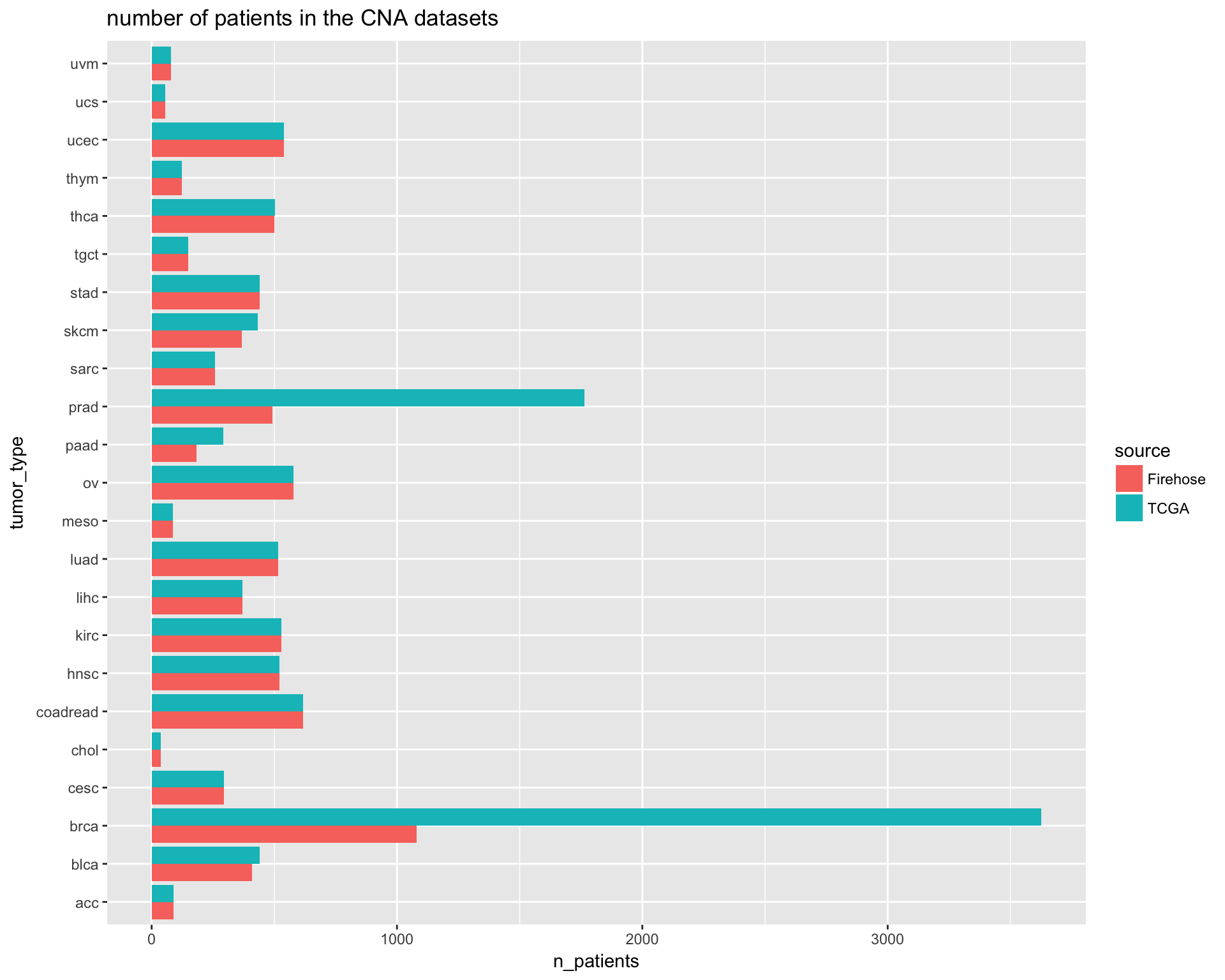
apply changes to the TCGA population object.
# Apply changes
TCGA_population@dataFull$copynumber <- copynumber
TCGA_population <- subsetAlterations(TCGA_population)
## Subsetting mutations...## Subsetting copynumber...Compare with Shiva population
In this section we will visualize a comparison between the samples available from the TCGA versus the samples in the SHIVA trial.
purrr::map2(
    .x = list( TCGA_population@dataFull$copynumber$Samples, SHIVA_population@dataFull$copynumber$Samples )
  , .y = list( "TCGA", "SHIVA" )
  , .f = ~ purrr::map_int(.x, length) %>%
      data.frame(n_patients = .) %>%
      tibble::rownames_to_column("tumor_type") %>%
      dplyr::mutate(source = .y)
  ) %>%
  dplyr::bind_rows() %>%
  ggplot(aes(reorder(tumor_type, n_patients), n_patients, fill=source)) +
    geom_bar(stat="identity", position= position_dodge()) +
    scale_fill_manual(values=MYPALETTE(10)[c(10,2)]) +
    coord_flip() +
    ggtitle("Number of samples available from TCGA and SHIVA group by tumor types")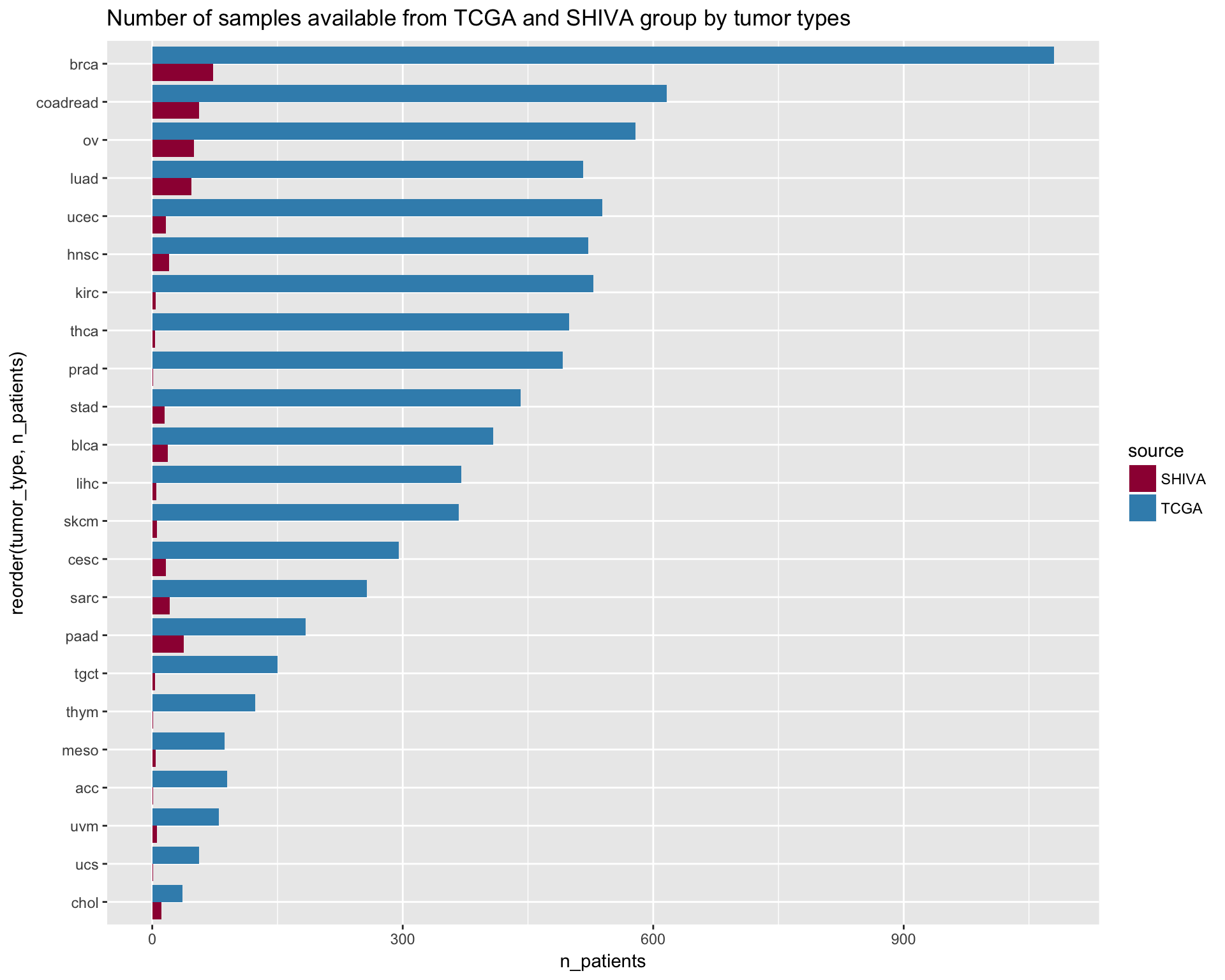
RESULTS - comparison between the TCGA population and SHIVA
- ANALYSIS 1) % of patients found to have an alteration that could be allocated to the targeted therapy group;
- ANALYSIS 2) Gene alteration frequency;
- ANALYSIS 3) Patient allocation;
- ANALYSIS 4) Power analysis of the study.
1. Detected Fraction
Detected Fraction TCGA population
One common question that is often considered when trying to design custom target enrichment panel, is the percentage of the population that would be “captured” by the design of the panel. The following plot shows the number of alteration (x-axis) found in the sample (patient) population (y-axis). The panel detected fraction can be defined as the number of patients with at least one alteration detectable by the genomic panel. In this simulation we are interested in comparing the detected fraction in the TCGA and SHIVA population. The TCGA population, will be corrected with a weighted bootstrap approach, to match the composition of the SHIVA population during recruitment.
# Run simulation
# ------------------------------------------------------------------------------
N_SIMULATIONS = 200

simul <- mclapply(1:N_SIMULATIONS , function(x) {
            cov <- coveragePlot(TCGA_population
                    , alterationType=c("mutations" , "copynumber")
                    , collapseByGene=TRUE
                    , tumor.weights = tumor_weights
                    , maxNumAlt = 7
                    , noPlot=TRUE
                     )
            return(cov$plottedTable/cov$Samples[1])
        } , mc.cores=4)

## Prepare function for plotting detected fraction with Confidenti intervals
# ------------------------------------------------------------------------------

# Convert to dataframe
simul <- data.frame(matrix(unlist(simul)
                        , nrow=length(simul)
                        , byrow=T )
                 , stringsAsFactors = FALSE)

# GET STATS
# ------------------------------------------------------------------------------
# Calculate for each n° of alteration, the mean
detectionPower <- colMeans(simul)

# Calculate lower CI for bootstrap
leftCI <- apply(simul,2,function(x){left <- quantile(x, 0.025)})

# Calculate upper CI for bootstrap
rightCI <- apply(simul,2,function(x){right <- quantile(x, 0.975)})

# Preapre for column with # alterations
n_alterations <- 1:length(detectionPower)

# Put them all together in a data frame
dtpow <- data.frame(n_alterations, detectionPower, leftCI, rightCI)

# Generate the plot
TCGA_detection_image <- dtpow %>%
  ggplot(aes(x=n_alterations, y=detectionPower)) +
  geom_bar(stat="identity" , position=position_dodge(), fill=MYPALETTE(10)[2]) +
  scale_y_continuous(limits = c(0,1)) +
  scale_x_continuous(breaks = n_alterations, trans = "reverse") +
  geom_errorbar(aes(ymax=rightCI
                    , ymin=leftCI)
                , position=position_dodge(0.9)
  ) +
  ggtitle("Overall detected fraction in TCGA Population") +
  annotate("text"
           , x=n_alterations
           , y=detectionPower+0.15
           , label= sapply(detectionPower*100
                           , function(x) paste(c(round(x, digits=2), "%")
                                               , collapse=" ")
           )
  ) +
  coord_flip()

# Show image
TCGA_detection_image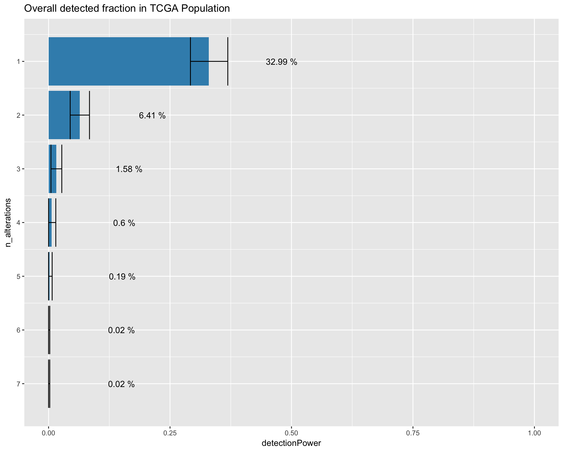
# Preview table
datatable_withbuttons(dtpow, caption = "detected fraction TCGA")
Contribution to the detected fraction allocated by alteration type.
Preview table with the contribution to the overall detected fraction by only mutation alterations.
# MUTATION CONTRIBUTIONS
# ------------------------------------------------------------------------------

simul <- mclapply(1:N_SIMULATIONS , function(x) {
            cov <- coveragePlot(TCGA_population
                    , alterationType=c("mutations")
                    , collapseByGene=TRUE
                    , tumor.weights = tumor_weights
                    , maxNumAlt = 7
                    , noPlot=TRUE
                     )
            return(cov$plottedTable/cov$Samples[1])
        } , mc.cores=4)

TCGA_detection_muts <- simulate_detectionPower_img(simul)

# Preview image
#TCGA_detection_muts + ggtitle("Mutation only detected fraction in TCGA")

# preview table
simulate_detectionPower_tbl(simul) %>%
  datatable_withbuttons(caption = "Mutation only detected fraction in TCGA")
Preview table with the contribution to the overall detected fraction by only CNA alteartions.
# COPYNUMBER CONTRIBUTION
# ------------------------------------------------------------------------------
simul <- mclapply(1:N_SIMULATIONS , function(x) {
            cov <- coveragePlot(TCGA_population
                    , alterationType=c("copynumber")
                    , collapseByGene=TRUE
                    , tumor.weights = tumor_weights
                    , maxNumAlt = 7
                    , noPlot=TRUE
                     )
            return(cov$plottedTable/cov$Samples[1])
        } , mc.cores=4)

TCGA_detection_cna <- simulate_detectionPower_img(simul)

# Preview image
#TCGA_detection_cna + ggtitle("CNA only detected fraction in TCGA")

# Preview table
simulate_detectionPower_tbl(simul) %>%
  datatable_withbuttons(caption = "CNA only detected fraction in TCGA")
Preview plot with the contribution to the overall detected fraction by only mutation and CNA alteartions seperately
gridExtra::grid.arrange(TCGA_detection_muts + ggtitle("detected fraction in TCGA: Mutation only")
                        , TCGA_detection_cna + ggtitle("detected fraction in TCGA: CNA only "))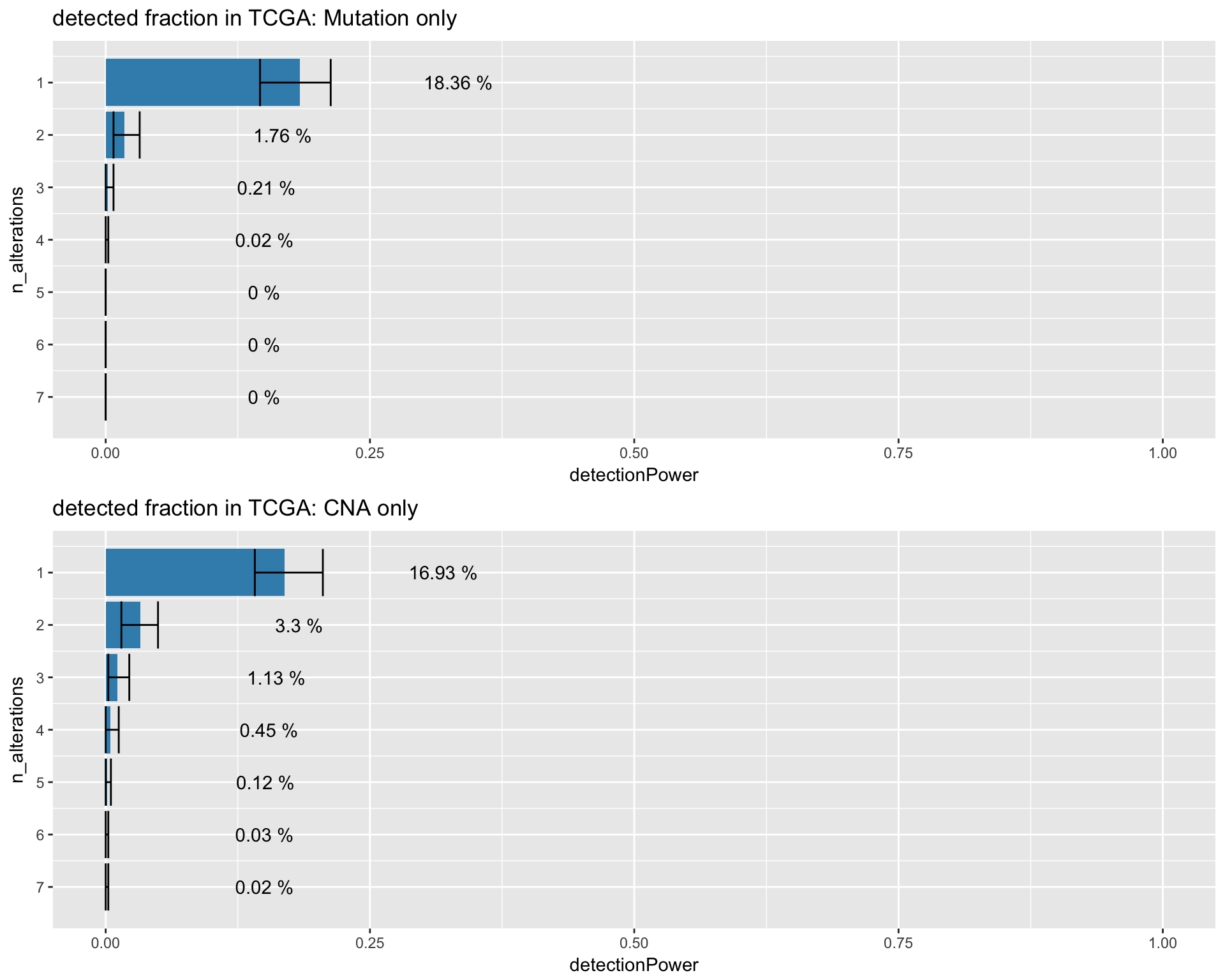
Detected fraction SHIVA population
# calculate shiva detected fraction
shiva_detect <-suppressWarnings(
                  coveragePlot(SHIVA_population
                   , alterationType = c("mutations", "copynumber")
                   , collapseByGene = TRUE
                   , maxNumAlt = 7
                   , noPlot= TRUE
                  )
              )

# calculate frequencies
shiva_freq <- as.numeric(shiva_detect$plottedTable/shiva_detect$Samples[1])

# Preapre for column with # alterations
n_alterations <- 1:length(shiva_freq)

# Put them all together in a data frame
dtpow_shiva <- data.frame(n_alterations, shiva_freq= shiva_freq)

# left CI and right CI
dtpow_shiva$leftCI <- purrr::map_dbl(shiva_freq, ~ leftCIprop(., sum(tumor_weights)))
dtpow_shiva$rightCI <- purrr::map_dbl(shiva_freq, ~ rightCIprop(., sum(tumor_weights)))

# Generate the plot
SHIVA_detection_image <- dtpow_shiva %>%
  ggplot(aes(x=n_alterations, y=shiva_freq)) +
    geom_bar(stat="identity" , position=position_dodge(), fill=MYPALETTE(10)[10]) +
    scale_y_continuous(limits = c(0,1)) +
    scale_x_continuous(breaks = n_alterations, trans = "reverse") +
    geom_errorbar(aes(   ymax= leftCI
                       , ymin= rightCI)
                   , position=position_dodge(0.9)
    ) +
    ggtitle("Detected fraction SHIVA population") +
    annotate("text"
             , x=n_alterations
             , y=shiva_freq+0.15
             , label= sapply(shiva_freq*100
                             , function(x) paste(c(round(x, digits=2), "%")
                                                 , collapse=" ")
             )
    ) +
    coord_flip()

#Export as a svg
#img_file = "../Figures/fig4B.svg"
#ggsave(filename=img_file, plot=SHIVA_detection_image, device = "svg")

# Show image
SHIVA_detection_image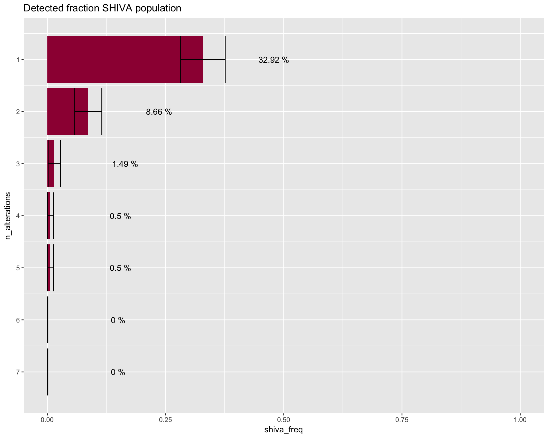
# Preview table
datatable_withbuttons(dtpow_shiva)
Contribution to the detected fraction allocated by alteration type.
coveragePlot(SHIVA_population
             , alterationType = c("mutations", "copynumber")
             , grouping = "alteration_id"
             #, noPlot=TRUE
             )
# SHIVA mutations ONLY
cov <- coveragePlot(SHIVA_population
             , alterationType = c("mutations")
             , grouping = "alteration_id"
             , noPlot=TRUE
             )
cov <- data.frame( cov$plottedTable / cov$Samples) %>%
  tidyr::gather(n_alterations, freq)

cov$leftCI <- purrr::map_dbl(cov$freq, ~ leftCIprop(., sum(tumor_weights)))
cov$rightCI <- purrr::map_dbl(cov$freq, ~ rightCIprop(., sum(tumor_weights)))

datatable_withbuttons(cov, caption="Datatable with detected fraction from Mutations for the SHIVA population")
# SHIVA copynumber ONLY
cov <- coveragePlot(SHIVA_population
, alterationType = c("copynumber")
, grouping = "alteration_id"
, noPlot=TRUE
)
cov <- data.frame( cov$plottedTable / cov$Samples) %>%
tidyr::gather(n_alterations, freq)
cov$leftCI <- purrr::map_dbl(cov$freq, ~ leftCIprop(., sum(tumor_weights)))
cov$rightCI <- purrr::map_dbl(cov$freq, ~ rightCIprop(., sum(tumor_weights)))
datatable_withbuttons(cov, caption="Datatable with detected fraction from CNA for the SHIVA population")Merge the detected fraction from the 2 population in one plot
fig4a <- gridExtra::grid.arrange(TCGA_detection_image, SHIVA_detection_image)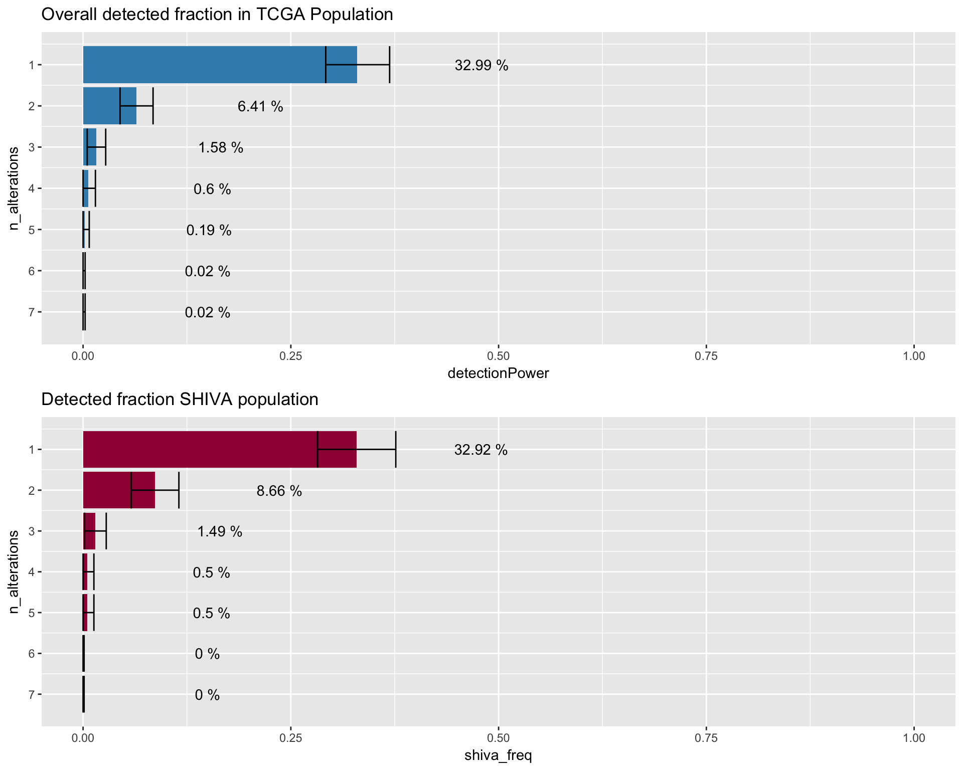
#Export as a svg
#img_file = "../Figures/fig4A.svg"
#ggsave(filename=img_file, plot=fig4a, device = "svg", width=10, height = 8)


# Preview image
fig4a
## TableGrob (2 x 1) "arrange": 2 grobs
## z cells name grob
## 1 1 (1-1,1-1) arrange gtable[layout]
## 2 2 (2-2,1-1) arrange gtable[layout]2. Gene alteration Frequency
In this section, we will compare each gene individually, for both CNA and Mutations.
SNV
###############################################################################
# Fetch SNV data from TCGA population
# -----------------------------------------------------------------------------
tcga_wide <- purrr::map(1:N_SIMULATIONS
           , ~ cpFreq(TCGA_population, alteration="mutations", tumor.weights = tumor_weights) %>%
                tidyr::spread(gene_symbol, freq)
           ) %>% bind_rows

# GET STATS
# ------------------------------------------------------------------------------
# Calculate for each n° of alteration, the mean
freq <- colMeans(tcga_wide)

# Calculate lower CI for bootstrap
leftCI <- apply(tcga_wide,2,function(x){left <- quantile(x, 0.025)})

# Calculate upper CI for bootstrap
rightCI <- apply(tcga_wide,2,function(x){right <- quantile(x, 0.975)})


# Put them all together in a data frame
tcga_snv <- data.frame(freq, leftCI, rightCI, population="TCGA") %>%
  tibble::rownames_to_column("gene")

###############################################################################
# Fetch CNA data from SHIVA population
# -----------------------------------------------------------------------------
temp <- cpFreq(SHIVA_population, alteration="mutations")
temp <- temp[which(temp[["gene_symbol"]] %in% SHIVA_population@arguments$panel$gene_symbol),]

# get CI
leftCI <- purrr::map_dbl(temp$freq, ~ leftCIprop(., sum(tumor_weights)))
rightCI <- purrr::map_dbl(temp$freq, ~ rightCIprop(., sum(tumor_weights)))

# get DF
shiva_snv <- temp %>%
  dplyr::rename(gene = gene_symbol) %>%
  dplyr::mutate(leftCI=leftCI
                , rightCI=rightCI
                ) %>%
  dplyr::mutate(population = "SHIVA")

###############################################################################
# put the plots together
# -----------------------------------------------------------------------------

# Put them together
merged_snv <- rbind(tcga_snv, shiva_snv)

# bind SHIVA and TCGA
fig4b <- merged_snv %>%
  dplyr::mutate(gene= factor(gene, levels = unique(gene[order(freq)]))) %>%
  ggplot(aes(x=gene, y=freq, fill=population)) +
  geom_bar(stat="identity", position=position_dodge()) +
  scale_fill_manual(values=MYPALETTE(10)[c(2,10)]) +
  #scale_y_continuous(limits = c(0,.7)) +
  geom_errorbar(aes(ymax=rightCI
                    , ymin=leftCI)
                , position=position_dodge(0.9)
  ) +
 ggtitle("SNV frequency comparison in the two populations") +
 coord_flip()


#img_file = "../Figures/fig4B.svg"
#ggsave(filename=img_file, plot=fig4b, device = "svg", width=10, height = 8)

# Preview
fig4b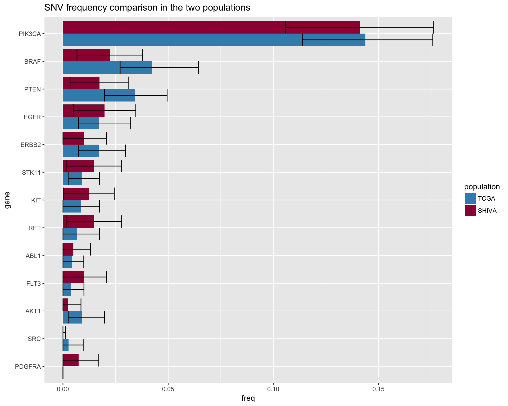
CNA
# Fetch CNA data from TCGA population
# ------------------------------------------------------------------------------
simul_amplifications <- lapply(1:50, function(x) {
            cpFreq(TCGA_population, alteration="copynumber", tumor.weights = tumor_weights) %>%
                dplyr::select(amplification) %>%
                tibble::rownames_to_column("gene") %>%
                tidyr::spread(gene, amplification)
        })

simul_amplifications <- simul_amplifications %>%  bind_rows()

simul_deletions <- lapply(1:50, function(x) {
            cpFreq(TCGA_population, alteration="copynumber", tumor.weights = tumor_weights) %>%
                dplyr::select(deletion) %>%
                tibble::rownames_to_column("gene") %>%
                tidyr::spread(gene, deletion)
        }) %>%  bind_rows()

# GET STATS
# ------------------------------------------------------------------------------
TCGA_amplifications_df <- get_bootstrap_stats(simul_amplifications) %>%
  tibble::rownames_to_column("gene") %>%
  dplyr::mutate(population = "TCGA")

TCGA_deletion_df <- get_bootstrap_stats(simul_deletions) %>%
  tibble::rownames_to_column("gene") %>%
  dplyr::mutate(population = "TCGA")


# Fetch CNA data from SHIVA population
# ------------------------------------------------------------------------------

# Amplifications
# ------------
shiva_cna_amplification <- cpFreq(SHIVA_population, alteration="copynumber") %>%
  tibble::rownames_to_column("gene") %>%
  dplyr::select(-deletion, -normal) %>%
  dplyr::rename(freq = amplification) %>%
  dplyr::mutate(population = "SHIVA")

# Calculate left CI and right CI
shiva_cna_amplification$leftCI <- purrr::map_dbl(shiva_cna_amplification$freq, ~ leftCIprop(., sum(tumor_weights)))
shiva_cna_amplification$rightCI <- purrr::map_dbl(shiva_cna_amplification$freq, ~ rightCIprop(., sum(tumor_weights)))

# last formattings
shiva_cna_amplification <-  shiva_cna_amplification %>%
  dplyr::mutate(row_counter = 1:nrow(shiva_cna_amplification)) %>%
  dplyr::select(gene, row_counter, freq, leftCI, rightCI, population)


# Deletion
# ------------
shiva_cna_deletion <- cpFreq(SHIVA_population, alteration="copynumber") %>%
  tibble::rownames_to_column("gene") %>%
  dplyr::select(-amplification, -normal) %>%
  dplyr::rename(freq = deletion) %>%
  dplyr::mutate(population = "SHIVA")

# Calculate left CI and right CI
shiva_cna_deletion$leftCI <- purrr::map_dbl(shiva_cna_deletion$freq, ~ leftCIprop(., sum(tumor_weights)))
shiva_cna_deletion$rightCI <- purrr::map_dbl(shiva_cna_deletion$freq, ~ rightCIprop(., sum(tumor_weights)))

# last formattings
shiva_cna_deletion <-  shiva_cna_deletion %>%
  dplyr::mutate(row_counter = 1:nrow(shiva_cna_deletion)) %>%
  dplyr::select(gene, row_counter, freq, leftCI, rightCI, population)

# Prepare filter
# Removed genes not considered in the panel for amplifications or deletions
# ------------
amplification_filter <- SHIVA_design %>%
  dplyr::filter(exact_alteration == "amplification") %>%
  dplyr::select(gene_symbol) %>%
  .[[1]] %>%
  as.character()

deletion_filter <- SHIVA_design %>%
  dplyr::filter(exact_alteration == "deletion") %>%
  dplyr::select(gene_symbol) %>%
  .[[1]] %>%
  as.character()


# Merge datasets
# ------------
merged_cna_amplifications <- rbind(TCGA_amplifications_df, shiva_cna_amplification) %>%
  dplyr::filter(gene %in% amplification_filter)
merged_cna_deletion <- rbind(TCGA_deletion_df, shiva_cna_deletion) %>%
  dplyr::filter(gene %in% deletion_filter)


# bind SHIVA and TCGA | Amplification
# -----
CNA_plot_amplification <- merged_cna_amplifications %>%
  dplyr::mutate(gene= factor(gene, levels = unique(gene[order(freq)]))) %>%
  ggplot(aes(x=gene, y=freq, fill=population)) +
  geom_bar(stat="identity", position=position_dodge()) +
  scale_fill_manual(values=MYPALETTE(10)[c(10,2)]) +
  #scale_y_continuous(limits = c(0,.7)) +
  geom_errorbar(aes(ymax=rightCI
                    , ymin=leftCI)
                , position=position_dodge(0.9)
  ) +
 ggtitle("CNA Amplification frequency comparison in the two populations") +
 coord_flip()


CNA_plot_deletion <- merged_cna_deletion %>%
  dplyr::mutate(gene= factor(gene, levels = unique(gene[order(freq)]))) %>%
  ggplot(aes(x=gene, y=freq, fill=population)) +
  geom_bar(stat="identity", position=position_dodge()) +
  scale_fill_manual(values=MYPALETTE(10)[c(10,2)]) +
  #scale_y_continuous(limits = c(0,.7)) +
  geom_errorbar(aes(ymax=rightCI
                    , ymin=leftCI)
                , position=position_dodge(0.9)
  ) +
 ggtitle("CNA Deletion frequency comparison in the two populations") +
 coord_flip()


# Make the plot
fig4c <- gridExtra::grid.arrange(CNA_plot_amplification, CNA_plot_deletion, ncol=1, heights = c(20,5))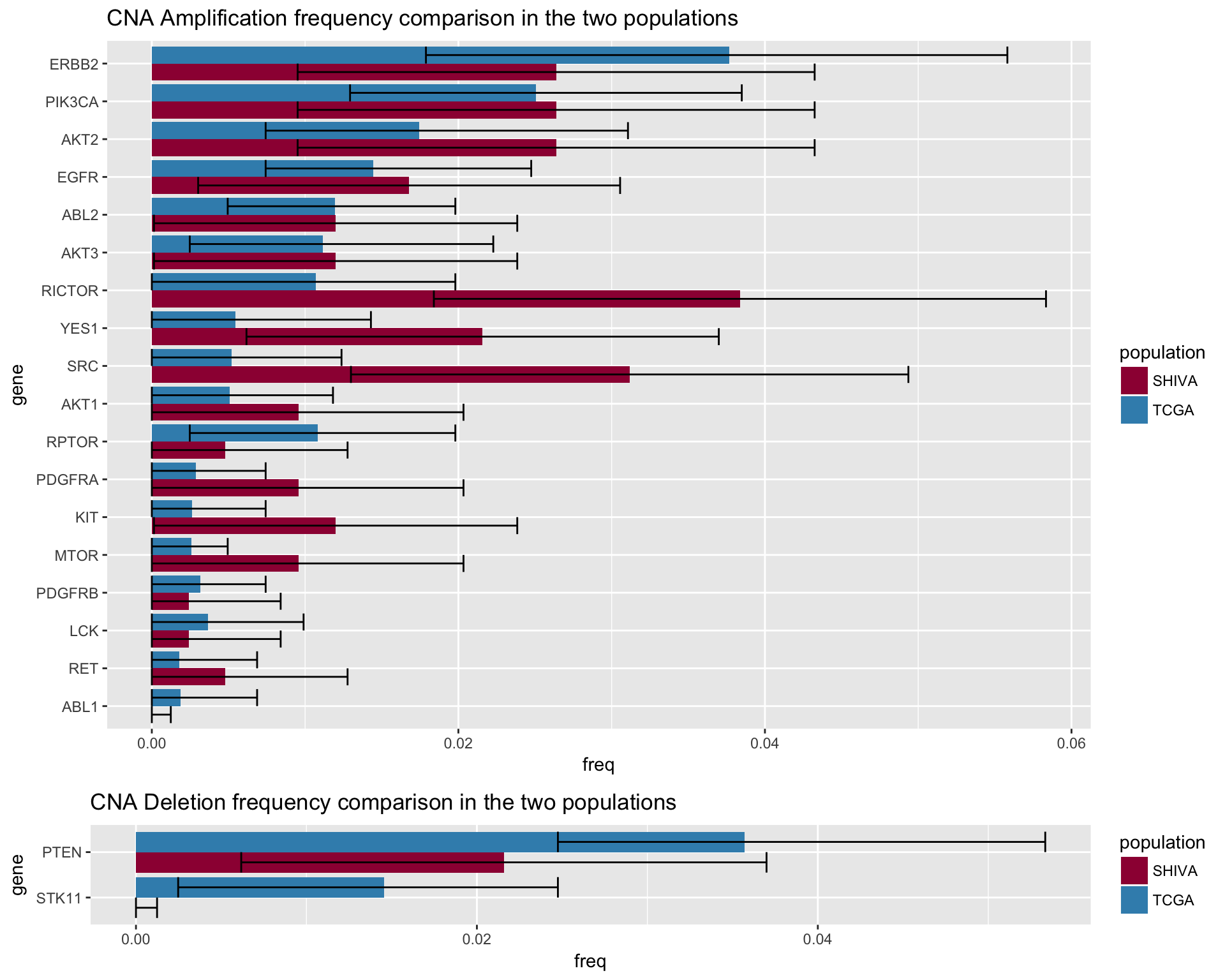
#Export as a svg
#img_file = "../Figures/fig4C.svg"
#ggsave(filename=img_file, plot=fig4c, device = "svg", width=10, height = 8)

# preview plot
fig4c
## TableGrob (2 x 1) "arrange": 2 grobs
## z cells name grob
## 1 1 (1-1,1-1) arrange gtable[layout]
## 2 2 (2-2,1-1) arrange gtable[layout]3. Patient allocation by pathway
In this part of the analysis we are comparing the patient allocation to the two molecular pathway threatments.
Show the maximum patient allocation to the molecular pathway threatmet. This is theoretical as, it presumes that one patient can be allocated to more than one treatment. There is infact a small percentage of patients with a set of alteration that makes them eligeble for both molecular treatmets.
# ##############################################################################
# Shiva population
# ##############################################################################
shiva_pathway <- coveragePlot(SHIVA_population
             , alterationType = c("mutations", "copynumber")
             , collapseByGene = TRUE
             , grouping = "group"
             , maxNumAlt = 1
             , noPlot = TRUE
             )

# calcualte frequency
shiva_pathway <- data.frame(shiva_pathway$plottedTable /shiva_pathway$Samples) %>%
  tibble::rownames_to_column("group") %>%
  dplyr::rename(allocation =X1)

# Calculate left CI and right CI
shiva_pathway$leftCI <- purrr::map_dbl(shiva_pathway$allocation, ~ leftCIprop(., sum(tumor_weights)))
shiva_pathway$rightCI <- purrr::map_dbl(shiva_pathway$allocation, ~ rightCIprop(., sum(tumor_weights)))

# transform table
shiva_allocation <- shiva_pathway %>%
  dplyr::mutate(row_counter = 1:n(), population = "SHIVA") %>%
  dplyr::select(group, row_counter, allocation, leftCI, rightCI, population)

# pepare plot
# shiva_allocation_img <- shiva_allocation %>%
#   ggplot(aes(x=row_counter, y=allocation, fill=group)) +
#     geom_bar(stat="identity" , position=position_dodge()) +
#     ggtitle("Shiva population pathway allocaiton frequency")

# Preview
#shiva_allocation_img
# ##############################################################################
# TCGA population
# ##############################################################################
simul <- mclapply(1:N_SIMULATIONS , function(x) {
# calculate allocated patients
cov <- coveragePlot(TCGA_population
, alterationType = c("mutations", "copynumber")
, collapseByGene = TRUE
, grouping = "group"
, maxNumAlt = 1
, tumor.weights = tumor_weights #tumor_weights
, noPlot=TRUE
)
# get frequency
as.data.frame(cov$plottedTable) %>%
tibble::rownames_to_column("group") %>%
dplyr::select(group, allocation= `1`) %>%
dplyr::mutate(allocation = allocation /cov$Samples[1]) %>%
tidyr::spread(group, allocation) %>%
return()
} , mc.cores=4) %>% bind_rows
# GET STATS
# ------------------------------------------------------------------------------
# Calculate for each n° of alteration, the mean
allocation <- apply(simul,2,mean)
# Calculate lower CI for bootstrap
leftCI <- apply(simul,2,function(x){left <- quantile(x, 0.025)})
# Calculate upper CI for bootstrap
rightCI <- apply(simul,2,function(x){right <- quantile(x, 0.975)})
# Preapre for column with the counter
row_counter <- 1:length(allocation)
# Put them all together in a data frame
tcga_allocation <- data.frame(row_counter, allocation, leftCI, rightCI, population="TCGA") %>%
tibble::rownames_to_column("group")
# Generate the Plot
# ------------------------------------------------------------------------------
# Generate the plot
# tcga_allocation_img <- tcga_allocation %>%
# ggplot(aes(x=row_counter, y=allocation, fill=group)) +
# geom_bar(stat="identity" , position=position_dodge()) +
# scale_y_continuous(limits = c(0,1)) +
# scale_x_continuous(breaks = row_counter, trans = "reverse") +
# geom_errorbar(aes(ymax=rightCI
# , ymin=leftCI)
# , position=position_dodge(0.9)
# ) +
# ggtitle("Patient Allocation to molecular pathway threatment") +
# annotate("text"
# , x=row_counter
# , y=allocation+0.15
# , label= sapply(allocation*100
# , function(x) paste(c(round(x, digits=2), "%")
# , collapse=" ")
# )
# ) +
# coord_flip()
# Preview
#tcga_allocation_img# ##############################################################################
# PLOT THEM TOGETHER
# ##############################################################################
merged_allocation <- rbind(shiva_allocation, tcga_allocation) %>%
dplyr::mutate(row_counter = 1:n())
fig4D <- merged_allocation %>%
ggplot(aes(x=group, y=allocation, fill=population)) +
geom_bar(stat="identity" , position=position_dodge()) +
scale_fill_manual(values=MYPALETTE(10)[c(10,2)]) +
scale_y_continuous(limits = c(0,.5)) +
ylab(label = "allocation frequency") +
facet_grid(. ~ group, space="free", scales="free") +
#scale_x_discrete(limits = merged_allocation$group) +
geom_errorbar(aes(ymax=rightCI
, ymin=leftCI)
, position="dodge"
) +
ggtitle("Patient Allocation to molecular pathway treatment, considering all the patients") +
geom_text(aes(label = sapply(allocation*100
, function(x) paste(c(round(x, digits=2), "%")
, collapse=" ")
)
) , position = position_dodge(width = 1)
, vjust = -6
) +
theme(axis.text.x=element_blank()
, axis.ticks.x= element_blank()
, axis.title.x = element_blank()
)
#Export as a svg
#img_file = "../Figures/fig4D.svg"
#ggsave(filename=img_file, plot=fig4D, device = "svg")
# Preview image
fig4D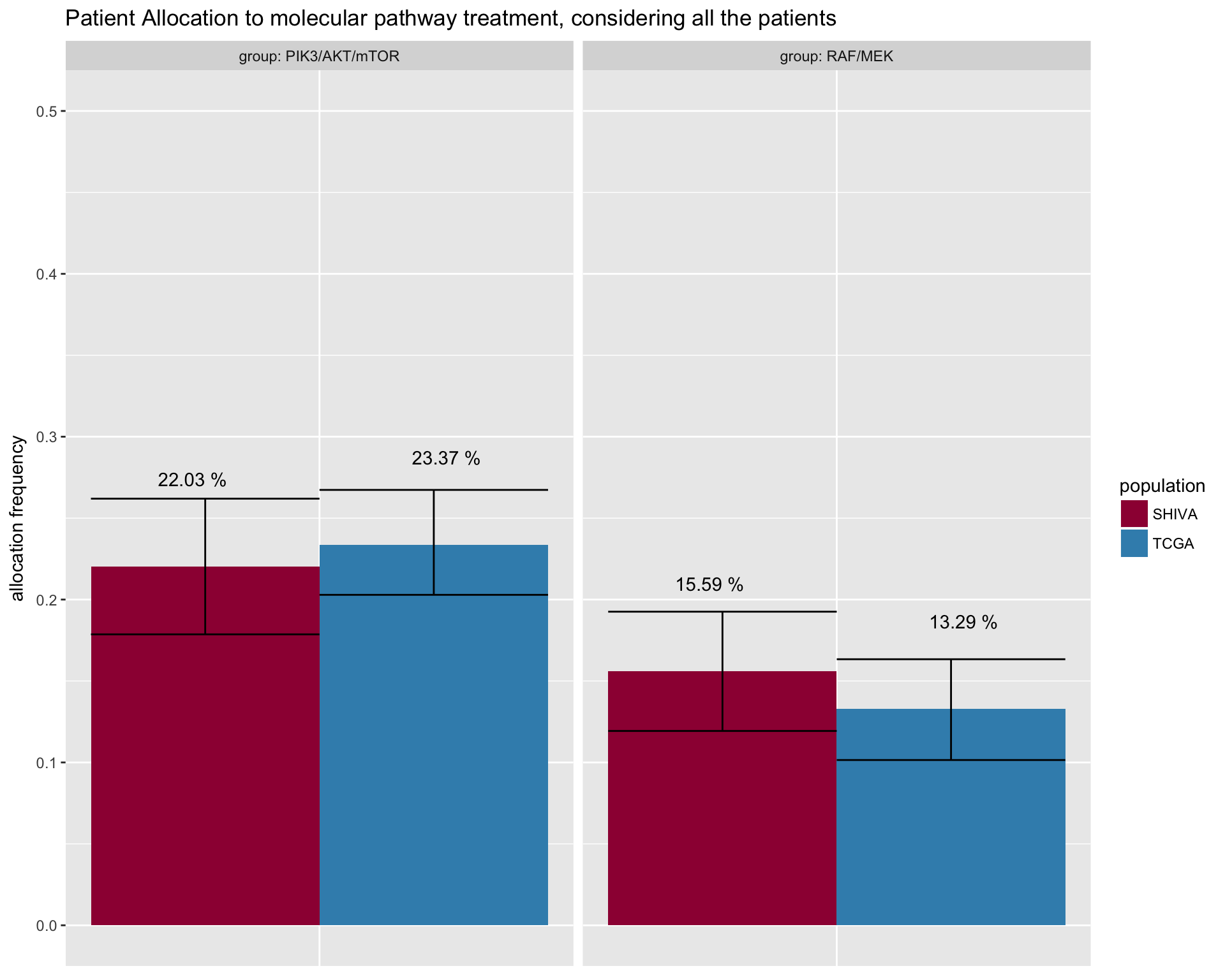
datatable_withbuttons(merged_allocation)Show patients eligible to both treatments separately
In case of a patient eligible for both molecular pathways treatment, the SHIVA medical board would decide in with cohord to allocate the patient. To allow a better comparison, the following plot separates the patients eligible to both treatments. The y-axes shows the tot number of patients that can be allocated in a molecular pathway treatmet.
# ALLOCATION FUNCTION with not predefined rule
# ------------------
# Create function to perform the following tasks:
# 1. extract a weighted (according to SHIVA population) sample from the population
# 2. Simulate patient allocation according the defined schema
allocate_patients_fn <- function(population, weights=FALSE){

  #extract patient data from the panel
  if(weights){
    patient_lt <- dataExtractor(population
                  , alterationType = c("copynumber", "mutations")
                  , collapseByGene = TRUE
                  , tumor.weights = weights
                  )
  } else {
    patient_lt <- dataExtractor(population
                  , alterationType = c("copynumber", "mutations")
                  , collapseByGene = TRUE
                  )
  }

  #select general dataframe
  patient_df <- patient_lt$data

  # replace / with _
  patient_df[,2] <- gsub("/", "_", patient_df[,2])

  # generate a frequency table that indicates, for each patient, elibibility to group allocation, as well as tumor_type
  # one patient per row.
  patient_allocation_df <- patient_df %>%
    dplyr::select(group, case_id, tumor_type) %>%
    dplyr::mutate(found = TRUE) %>%
    unique() %>%
    tidyr::spread(group, found)

  # SIMULATE PATIENTS ALLOCATION ACCORDING TO A SPECIFIC ORDER
  # ----------------------------------------
  # select ONLY PIK3_AKT_mTOR compatible patients
  PIK3_AKT_mTOR_assigned <- patient_allocation_df %>%
    dplyr::filter(is.na(RAF_MEK)) %>%
    dplyr::filter(PIK3_AKT_mTOR == TRUE)

  # select ONLY RAF_MEK compatible patients
  RAF_MEK_assigned <- patient_allocation_df %>%
    dplyr::filter(is.na(PIK3_AKT_mTOR)) %>%
    dplyr::filter(RAF_MEK == TRUE)

  # Select patients that would be allocated to either
  eligible_both <- patient_allocation_df %>%
    dplyr::filter(RAF_MEK == TRUE) %>%
    dplyr::filter(PIK3_AKT_mTOR == TRUE)

  # freq of patient allocation in each treatment group
  df <- data.frame(PIK3_AKT_mTOR = nrow(PIK3_AKT_mTOR_assigned) / nrow(patient_allocation_df)
             , RAF_MEK = nrow(RAF_MEK_assigned) / nrow(patient_allocation_df)
             , eligible_both = nrow(eligible_both) / nrow(patient_allocation_df)
  )
  return(df)
}
# TCGA
# ------------------------------------------------------------------------------
bootstrapping_df <- replicate(500
, allocate_patients_fn(TCGA_population, tumor_weights)
, simplify=FALSE
) %>% do.call("rbind", .)
# calculae the mean, sd and CI for each treatment group
bootstrappingMeans <- colMeans(bootstrapping_df)
lowerCI <- apply( bootstrapping_df , 2 , function(x) quantile(x, 0.025))
upperCI <- apply( bootstrapping_df , 2 , function(x) quantile(x, 0.975))
# Prepare dataframe for plotting
# ----------------------------
# covert to dataframe
tcga_df <- data.frame(mean=bootstrappingMeans
, lowerSD = NA
, upperSD = NA
, lowerCI = lowerCI
, upperCI = upperCI
) %>%
tibble::rownames_to_column("group_treatment") %>%
dplyr::arrange(mean) %>%
dplyr::mutate(dataset="TCGA")
# SHIVA
# ------------------------------------------------------------------------------
shiva_df <- allocate_patients_fn(SHIVA_population) %>%
tidyr::gather(group_treatment, mean) %>%
dplyr::mutate(lowerSD = NA
, upperSD = NA
, lowerCI = leftCIprop(mean, sum(tumor_weights))
, upperCI = rightCIprop(mean, sum(tumor_weights))
, dataset = "SHIVA"
)
# merge dataframes together
merge_df <- rbind(shiva_df, tcga_df) %>%
dplyr::rename(freq = mean)
# ----------------------------
# PLOT2 - Same side barplot
# barplot, with only the genes in the panel
fig4E <- merge_df %>%
dplyr::mutate(origin=paste(as.character(group_treatment), as.character(dataset), sep=":")) %>%
dplyr::mutate(row_counter = as.integer(factor(dataset, labels = c(0,1)))) %>%
ggplot(aes(x=origin, y=freq, fill=dataset)) +
geom_bar(stat="identity") +
scale_fill_manual(values=MYPALETTE(10)[c(10,2)]) +
geom_errorbar(aes(min=lowerCI, max=upperCI)) +
facet_grid(. ~ group_treatment, space="free", scales="free") +
theme(axis.text.x=element_blank()
, axis.ticks.x= element_blank()
, axis.title.x = element_blank()
) +
labs(title="Comparison between expected allocation to molecular pathways")
fig4E <- fig4E + geom_text(aes(x=(row_counter)
, y=upperCI+.05
, label= sapply(freq*100
, function(x) paste(c(round(x, digits=2), "%")
, collapse=" ")
)
)
)
#Export as a svg
#img_file = "../Figures/fig4E.svg"
#ggsave(filename=img_file, plot=fig4E, device = "svg", width=10, height = 8)
# preview image
fig4E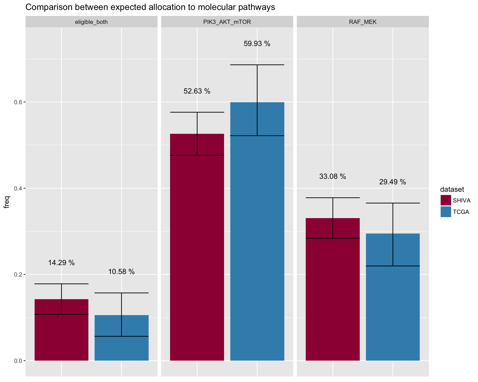
merge_df %>%
  dplyr::select(-lowerSD, -upperSD) %>%
  datatable_withbuttons
################################################################################
# ADD plot by Drug
################################################################################
# get the numer of samples used for the next computation
n_samples <- coveragePlot(TCGA_population
, alterationType=c("mutations" , "copynumber")
, collapseByGene=TRUE
, tumor.weights = tumor_weights
, maxNumAlt = 1
, noPlot=TRUE
, grouping = "drug"
)$Sample[1]
# TCGA
# ------------------------------------------------------------------------------
bootstrapping_df <- replicate(500
, coveragePlot(TCGA_population
, alterationType=c("mutations" , "copynumber")
, collapseByGene=TRUE
, tumor.weights = tumor_weights
, maxNumAlt = 1
, noPlot=TRUE
, grouping = "drug"
) %>%
.$plottedTable %>%
data.frame %>%
tibble::rownames_to_column("drug") %>%
dplyr::rename(count=X1) %>%
dplyr::mutate(freq = count/n_samples) %>%
dplyr::select(-count) %>%
dplyr::mutate(drug= gsub( "drug: ", "", drug) ) %>%
tidyr::spread(drug, freq) %>%
dplyr::mutate(Sorafenib = if (exists('Sorafenib', where = .)) Sorafenib else 0) %>%
dplyr::mutate(Dasatinib = if (exists('Dasatinib', where = .)) Dasatinib else 0)
, simplify=FALSE
) %>% do.call("rbind", .)
# calculae the mean, sd and CI for each treatment group
bootstrappingMeans <- colMeans(bootstrapping_df)
lowerCI <- apply( bootstrapping_df , 2 , function(x) quantile(x, 0.025))
upperCI <- apply( bootstrapping_df , 2 , function(x) quantile(x, 0.975))
# Prepare dataframe for plotting
# ----------------------------
# covert to dataframe
tcga_df <- data.frame(mean=bootstrappingMeans
, lowerSD = NA
, upperSD = NA
, lowerCI = lowerCI
, upperCI = upperCI
) %>%
tibble::rownames_to_column("group_treatment") %>%
dplyr::arrange(mean) %>%
dplyr::mutate(dataset="TCGA")
# SHIVA
# ------------------------------------------------------------------------------
shiva_df <- coveragePlot(SHIVA_population
, alterationType=c("mutations" , "copynumber")
, collapseByGene=TRUE
, tumor.weights = tumor_weights
, maxNumAlt = 1
, noPlot=TRUE
, grouping = "drug"
) %>% .$plottedTable %>%
data.frame %>%
tibble::rownames_to_column("drug") %>%
dplyr::rename(count=X1) %>%
dplyr::mutate(freq = count/n_samples) %>%
dplyr::select(-count) %>%
dplyr::mutate(drug= gsub( "drug: ", "", drug) ) %>%
tidyr::spread(drug, freq) %>%
dplyr::mutate(Sorafenib = if (exists('Sorafenib', where = .)) Sorafenib else 0) %>%
dplyr::mutate(Dasatinib = if (exists('Dasatinib', where = .)) Dasatinib else 0) %>%
tidyr::gather(group_treatment, mean) %>%
dplyr::mutate(lowerSD = NA
, upperSD = NA
, lowerCI = map_dbl(mean, ~ leftCIprop(., sum(tumor_weights)))
, upperCI = map_dbl(mean, ~ rightCIprop(., sum(tumor_weights)))
, dataset = "SHIVA"
)
# merge dataframes together
merge_df <- rbind(shiva_df, tcga_df) %>%
dplyr::rename(freq = mean) %>%
mutate_cond(group_treatment %in% "Lapatinib+Trastuzumab", group_treatment = "Lapatinib+\nTrastuzumab")
# ----------------------------
# PLOT2 - Same side barplot
# barplot, with only the genes in the panel
fig4F <- merge_df %>%
dplyr::mutate(origin=paste(as.character(group_treatment), as.character(dataset), sep=":")) %>%
dplyr::mutate(row_counter = as.integer(factor(dataset, labels = c(0,1)))) %>%
ggplot(aes(x=origin, y=freq, fill=dataset)) +
geom_bar(stat="identity") +
scale_fill_manual(values=MYPALETTE(10)[c(10,2)]) +
geom_errorbar(aes(min=lowerCI, max=upperCI)) +
facet_grid(. ~ group_treatment, space="free", scales="free") +
theme(axis.text.x=element_blank()
, axis.ticks.x= element_blank()
, axis.title.x = element_blank()
) +
labs(title="Comparison between expected allocation to molecular pathways")
# +
# coord_flip()
#Export as a svg
#img_file = "../Figures/fig4F.svg"
#ggsave(filename=img_file, plot=fig4F, device = "svg")
# Preview
fig4F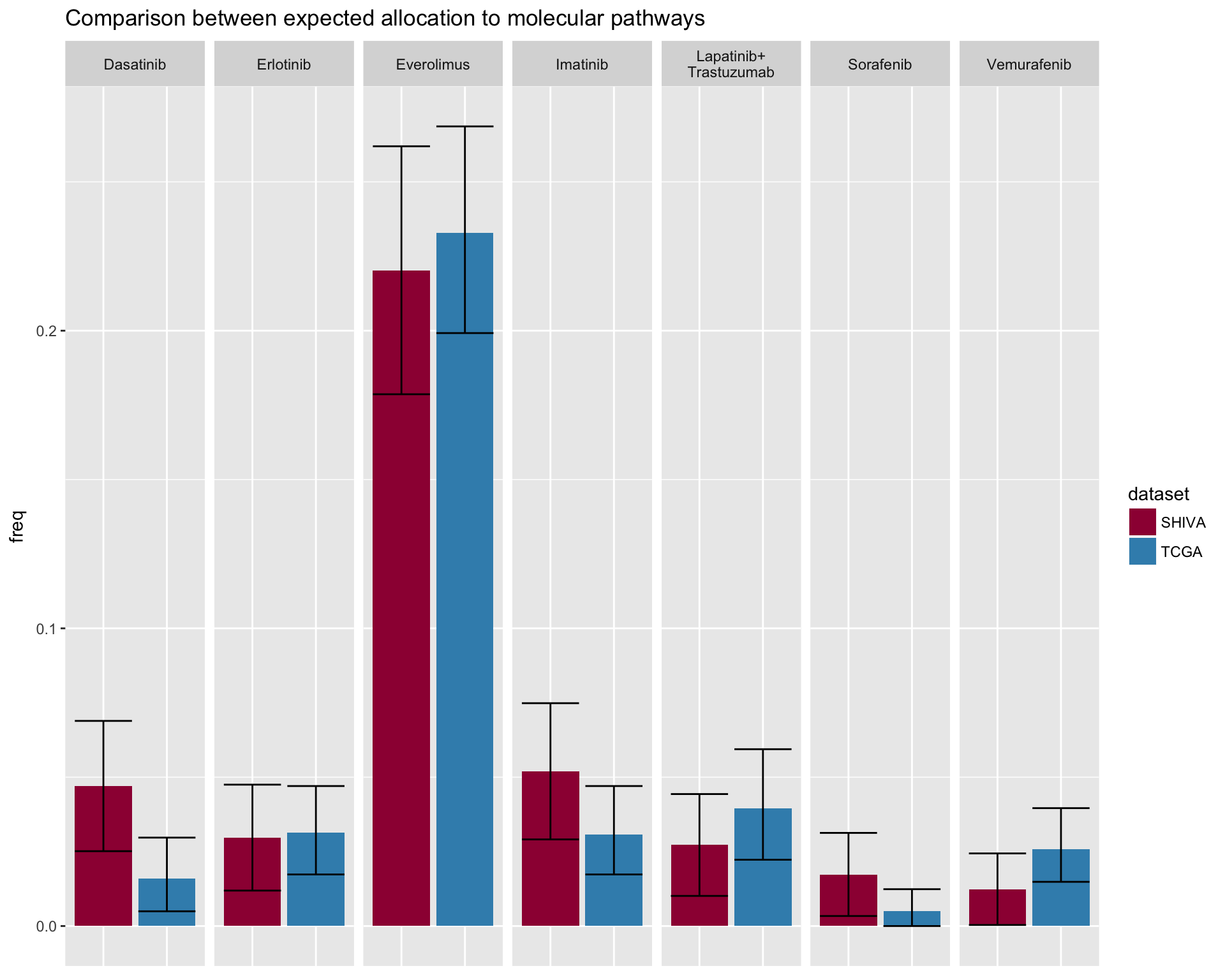
# preview table
merge_df %>%
  dplyr::select(-lowerSD, -upperSD) %>%
  datatable_withbuttons()
4. Power analysis
In this section we will calculate the sample size required for the SHIVA trial and our TCGA approximation. We first compare the sample size calculated on both populations on a full design with no granularity on the drug target. Basically a design to answer the question “target therapy VS standard of care”
Full Design
SHIVA
# Shiva full design
survPowerSampleSize(SHIVA_population
                    , alterationType = c("mutations", "copynumber")
                    , HR = 0.625
                    , power = seq(0.6 , 0.9 , 0.1)
                    , alpha = 0.05
                    , case.fraction = 0.5
                    #, tumor.freqs = tumor_freq
) + xlim(c(200,1000))
TCGA
survPowerSampleSize(TCGA_population
                    , alterationType = c("mutations", "copynumber")
                    , HR = 0.625
                    , power = seq(0.6 , 0.9 , 0.1)
                    , alpha = 0.05
                    , case.fraction = 0.5
                    , tumor.freqs = tumor_freq
) + xlim(c(200,1000))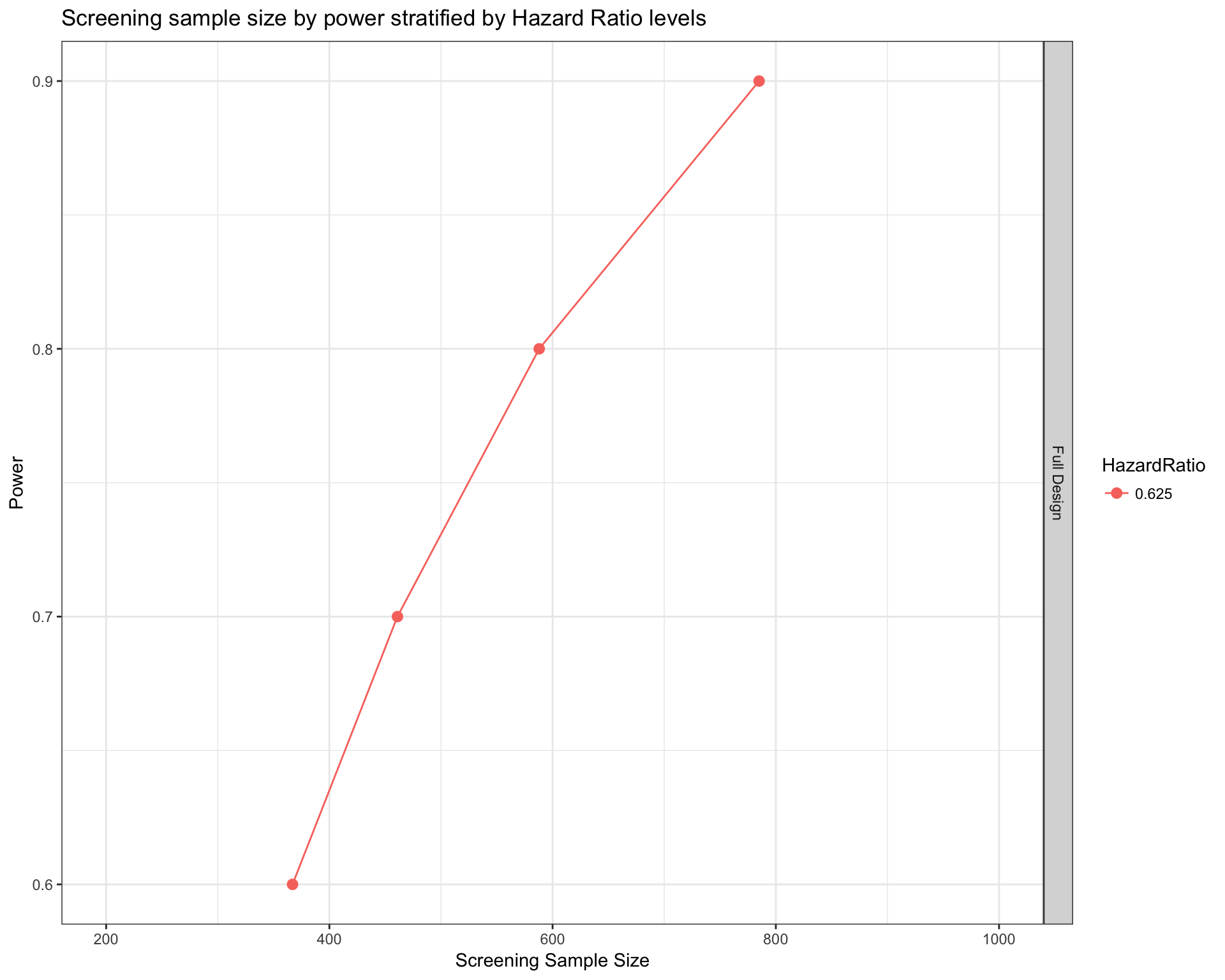
Comparison
tcgaFullDesign <- survPowerSampleSize(TCGA_population
                    , alterationType = c("mutations", "copynumber")
                    , HR = 0.625
                    , power = seq(0.6 , 0.9 , 0.1)
                    , alpha = 0.05
                    , case.fraction = 0.5
                    , tumor.freqs = tumor_freq
                    , noPlot = TRUE)[ , c("EligibleSampleSize" , "ScreeningSampleSize")]
shivaFullDesign <- survPowerSampleSize(SHIVA_population
                    , alterationType = c("mutations", "copynumber")
                    , HR = 0.625
                    , power = seq(0.6 , 0.9 , 0.1)
                    , alpha = 0.05
                    , case.fraction = 0.5
                    #, tumor.freqs = tumor_freq
                    , noPlot = TRUE)[ , c("EligibleSampleSize" , "ScreeningSampleSize")]
fullDesignComparison <- data.frame(ScreeningSampleSize_TCGA = tcgaFullDesign$ScreeningSampleSize
                                , ScreeningSampleSize_SHIVA = shivaFullDesign$ScreeningSampleSize
                                , EligibleSampleSize = shivaFullDesign$EligibleSampleSize
                                , Beta = 1 - seq(0.6 , 0.9 , 0.1)
                                , Power = seq(0.6 , 0.9 , 0.1)
                                , HR = 0.625)
datatable_withbuttons(fullDesignComparison)
The difference is very small. Just 2 patients at a 80% power.
Design by single drug category
Now we want to calculate sample size by each drug separately. This in not an optimal design since it relies on the assumption of indipendent studies. From this point on we will use the same value used in the design of the SHIVA trial:
- power 80%
- alpha 5%
- case.fraction 50%
- baseline event rate (ber) 85%
- average follow-up time 1.883
From the original publication:
The objective of the study was to detect a difference in progression-free survival between the treatment groups. Expected 6-month progression-free survival in the control group was 15%. We postulated that the experimental group would have 40% longer progression-free survival than that of the control group (hazard ratio [HR] 0·625). A total of 142 events was needed to detect a statistically significant difference with a type I error rate of 5% and a power of 80% in a two-sided setting. To be able to see these events, we planned to include a total of 200 patients.
SHIVA
shivaByDrug <- survPowerSampleSize(SHIVA_population
   , alterationType = c("mutations", "copynumber")
   , HR = 0.625
   , power = 0.8
   , alpha = 0.05
   , case.fraction = 0.5
   , ber=0.85
   , fu=1.883
   #, tumor.freqs = tumor_freq
   , var = "group"
   , noPlot=TRUE)

datatable_withbuttons(shivaByDrug)
TCGA
tcgaByDrug <- survPowerSampleSize(TCGA_population
   , alterationType = c("mutations", "copynumber")
   , HR = 0.625
   , power = 0.8
   , alpha = 0.05
   , case.fraction = 0.5
   , ber=0.85
   , fu=1.883
   , tumor.freqs = tumor_freq
   , var = "group"
   , noPlot=TRUE)

datatable_withbuttons(tcgaByDrug)
Design by drug: optimized
With our tool, we are also able to optimize the number of patients needed to be screened in order to assure a minimum of 80% power to all the arms of the study. We call this option priority trial and is basically a cascade design that tries to estimate a total sample size at screening that is sufficient to cover all the arms of the study with the desired power.
We run the TCGA population first.
TCGA
tcgaSimul <- mclapply(1:100 , function(x) {
    survPowerSampleSize(TCGA_population
        , alterationType = c("mutations", "copynumber")
        , HR = 0.625
        , power = 0.8
        , alpha = 0.05
        , ber=0.85
        , fu=1.883
        , case.fraction = 0.5
        , collapseByGene=TRUE
        , tumor.weights = tumor_weights
        , var = "group"
        , noPlot=TRUE
        , priority.trial=c("PIK3/AKT/mTOR", "RAF/MEK")
        , priority.trial.order="optimal")$'HR:0.625 | HR0:1 | Power:0.8'$Summary
    } , mc.cores=4)


summaryMat <- tcgaSimul[[1]]
for(i in rownames(summaryMat)){
    for(j in colnames(summaryMat)){
        vec <- sapply(tcgaSimul , function(x) x[i , j])
        summaryMat[i , j] <- paste(mean(vec) ,
                paste0( "(" , quantile(vec , 0.025)
                        , "-"
                        , quantile(vec , 0.975) , ")"))
    }
}
knitr::kable(summaryMat)| RAF/MEK | PIK3/AKT/mTOR | Total | |
|---|---|---|---|
| Screened | 1507.05 (1182.15-1939.15) | 0 (0-0) | 1507.05 (1182.15-1939.15) |
| Eligible | 199 (199-199) | 296.51 (214.95-413.675) | 495.51 (413.95-612.675) |
| Not.Eligible | 1012.53 (760.175-1369.525) | 0 (0-0) | 1012.53 (760.175-1369.525) |
The table above represents our cascade design starting from upper left. The first row is the recruitment row: number of new patients that need to be sequenced to obtain the required power. The left and right Confidence Intervals from the bootstrap simuation are indicated in parentesis. Starting by recruiting 1507.05 (1182.15-1939.15) for the most rare drug category (RAF/MEK) we will obtain on average 199 (199-199) eligible patients and discarding 1012.53 (760.175-1369.525) (the former are the patients not eligible to any molecular drug treatments). The non eligible patients of RAF/MEK might be eligible for other drug categories, so we calculate whether within these patients, there is an enough number of eligible patients to reach the required power. In case the number is sufficient, the algorithm indicates how many more patients are necessary to recruit. Based on our calculations no further patientes are necessary.
Finally, the last column indicates the total number of patients screened, eligible, and non eligible.
Starting from the most rare drug, we assure the minimum number of recruited patients that guarantee at least 80% power for each drug and the whole study.
SHIVA
With the SHIVA population we are going to check if the value obtained is compatible with the confidence interval calculated on TCGA data.
shivaSimul <- survPowerSampleSize(SHIVA_population
        , alterationType = c("mutations", "copynumber")
        , HR = 0.625
        , power = 0.8
        , alpha = 0.05
        , ber=0.85
        , fu=1.883
        , case.fraction = 0.5
        , collapseByGene=TRUE
        #, tumor.weights = tumor_weights
        , var = "group"
        , noPlot=TRUE
        , priority.trial=c("PIK3/AKT/mTOR", "RAF/MEK")
        , priority.trial.order="optimal")$'HR:0.625 | HR0:1 | Power:0.8'$Summary

knitr::kable(shivaSimul)| RAF/MEK | PIK3/AKT/mTOR | Total | |
|---|---|---|---|
| Screened | 1277 | 0 | 1277 |
| Eligible | 199 | 222 | 421 |
| Not.Eligible | 857 | 0 | 857 |
The number of recruited patients is compatible.
Post-hoc power of the SHIVA trial
We analyze now retrospectively the power of the SHIVA study under our framework by using the same number of patients reported in the publication. From text and Table 1 of the SHIVA publication:
- 496 Patients with a complete profile entered in the study
- 203 NOT eligible
- 293 eligible
- 46 (molecularly target) + 43 (physician’s choice) = 89 in PI3K/AKT/mTOR pathway arm
- 13 (molecularly target) + 11 (physician’s choice) = 24 in RAF/MEK pathway arm
Overall Power
In the design of a target therapy VS standard of care trial, we can simply check what is the resulting power of plugging-in 496 in our survPowerSampleSize function:
phPower <- survPowerSampleSize(SHIVA_population
                    , alterationType = c("mutations", "copynumber")
                    , HR = 0.625
                    , power = NULL
                    , sample.size = 496
                    , alpha = 0.05
                    , ber=0.85
                    , fu=1.883
                    , case.fraction = 0.5
                    , noPlot=TRUE)
knitr::kable(phPower)| Var | ScreeningSampleSize | EligibleSampleSize | Beta | Power | HazardRatio |
|---|---|---|---|---|---|
| Full Design | 496 | 164 | 0.2792024 | 0.7207976 | 0.625 |
A cohort of 496 individuals can guarantee a power of 0.72 with an eligible sample size of 164. The reason for the discrepancy with the eligible size of the original SHIVA study is the lack of the entire Hormone arm that decreases the detected fraction in this analysis. The entire study reaches this power but do not guarantees that each single arm has the same power level.
Optimized power
As mentioned before, the option priority.trial allows us to calculate an optimal sample size so that each arm reaches at least the desired power. Unfortunately, the option is not available yet to calculate post-hoc power given a sample size. We therefore try to calculate the post-hoc power by optimization. The idea is to calculate various sample sizes for different power levels to get a value equal or close enough to our 496.
First, create a function to optimize. This function takes a power level as input and returns the difference between the calculated sample size and 496 in absolute value.
powerOptimizer <- function(mypower){
  simul <- suppressWarnings(suppressMessages(
    survPowerSampleSize(SHIVA_population
        , alterationType = c("mutations", "copynumber")
        , HR = 0.625
        , power = mypower # only moving parameter, the rest is constant
        , alpha = 0.05
        , ber=0.85
        , fu=1.883
        , case.fraction = 0.5
        , collapseByGene=TRUE
        #, tumor.weights = tumor_weights
        , var = "group"
        , noPlot=TRUE
        , priority.trial=c("PIK3/AKT/mTOR", "RAF/MEK")
        , priority.trial.order="optimal")))
  # Return only the calculated Total Screened sample size
  out <- simul[[1]][1]$Summary["Screened" , "Total"]
  # Actual value to minimize is the absolute difference (we want to get close to 0)
  return( abs(496-out))
}
Let’s try some power values to see how this function behaves.
mypowers <- seq(0.1 , 0.8 , 0.05)
mySampSizeDiff <- sapply(mypowers , powerOptimizer)
plot(mypowers , mySampSizeDiff , pch=20 , col="black")
lines(mypowers , mySampSizeDiff , col="red")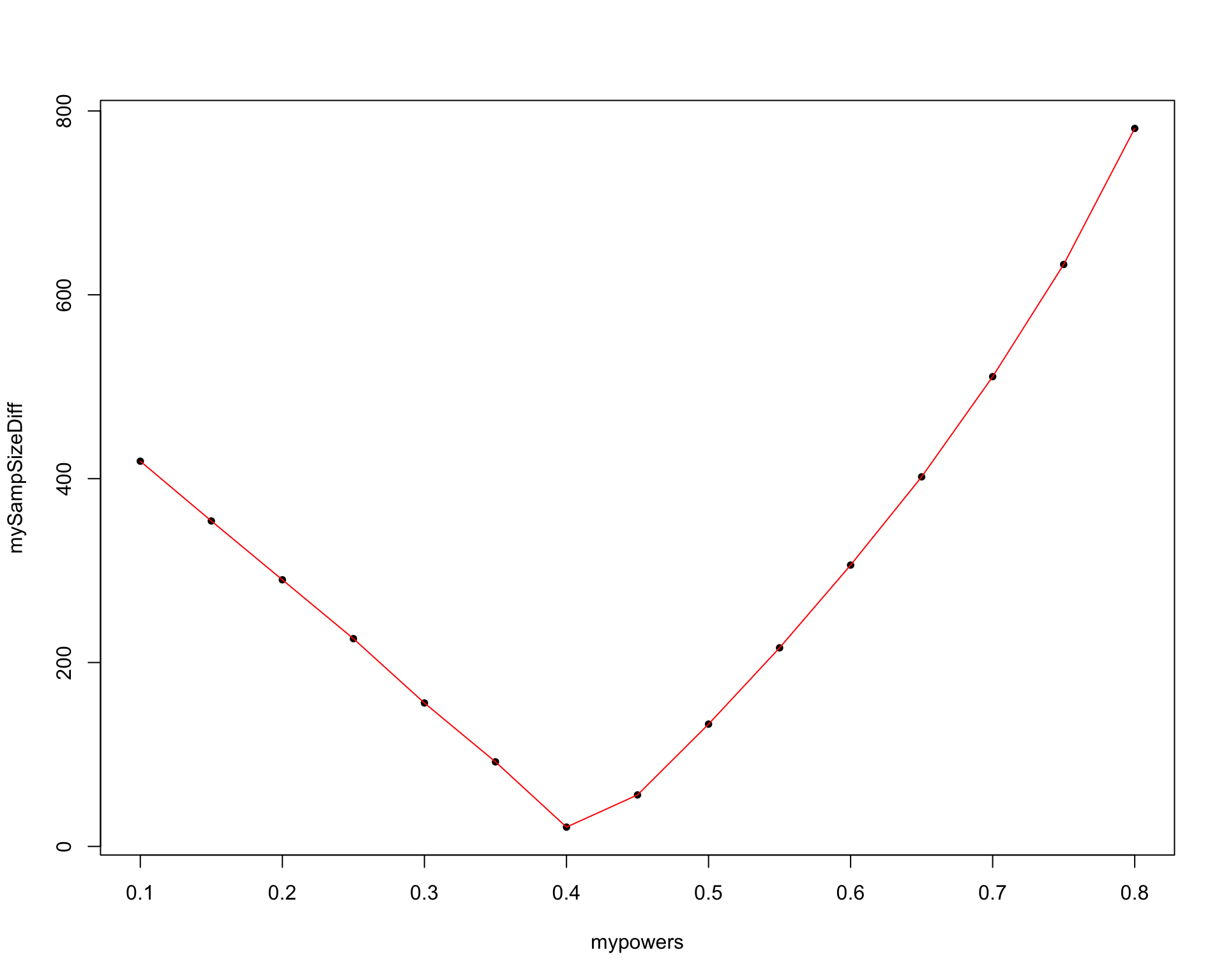
It’s pretty clear that we have a minimum at 0.4 when the sample size calculated is equal to 517. This function is clearly convex in the interval (0-1) of the possible power levels, so the post-hoc power resides between 0.35 and 0.45 (according to our plot points).
For a more robust optimization, we are going to use a linear optimizer. To facilitate the process, we will inizialize a value of 0.4 and lower and upper bounds of 0.35 and 0.45 (as calculated by our graphical method)
Since we are dealing with a one-dimentional problem with box constrains, we are going to use the Brent method.
myPHPoptim <- optim(par = 0.4 , fn = powerOptimizer
                  , lower = 0.35 , upper = 0.45 , method="Brent")

myPHPoptim
## $par
## [1] 0.4105573
##
## $value
## [1] 2
##
## $counts
## function gradient
## NA NA
##
## $convergence
## [1] 0
##
## $message
## NULLThe value of the slot convergence is telling us that the method worked. The actual power that can be reached by a 496 individuals study is just 41.0557295 for each single arm and it’s the reason why the SHIVA trial probably failed at demonstrating a difference between genomic therapy and standard of care.
By plugging in our value, we can see that:
plugInSampleSize <- survPowerSampleSize(SHIVA_population
        , alterationType = c("mutations", "copynumber")
        , HR = 0.625
        , power = myPHPoptim$par
        , alpha = 0.05
        , ber=0.85
        , fu=1.883
        , case.fraction = 0.5
        , collapseByGene=TRUE
        #, tumor.weights = tumor_weights
        , var = "group"
        , noPlot=TRUE
        , priority.trial=c("PIK3/AKT/mTOR", "RAF/MEK")
        , priority.trial.order="optimal")[[1]][1]$Summary
##
## Minimum Eligible Sample Size to reach 41% of power with an HR equal to 0.625 and a HR0 equal to 1 for each group is equal to: 77knitr::kable(plugInSampleSize)| RAF/MEK | PIK3/AKT/mTOR | Total | |
|---|---|---|---|
| Screened | 494 | 0 | 494 |
| Eligible | 77 | 86 | 163 |
| Not.Eligible | 332 | 0 | 332 |
So with an approximated screened sample size of 494 we obtain 163 eligible patients divided in 77 for RAF/MEK pathway arm and 86 for PIK3/AKT/mTOR pathway arm.
Session info
For reproducibility purpose:
sessionInfo()## R version 3.5.0 Patched (2018-06-01 r74839)
## Platform: x86_64-apple-darwin15.6.0 (64-bit)
## Running under: macOS High Sierra 10.13.3
##
## Matrix products: default
## BLAS: /Library/Frameworks/R.framework/Versions/3.5/Resources/lib/libRblas.0.dylib
## LAPACK: /Library/Frameworks/R.framework/Versions/3.5/Resources/lib/libRlapack.dylib
##
## locale:
## [1] en_US.UTF-8/en_US.UTF-8/en_US.UTF-8/C/en_US.UTF-8/en_US.UTF-8
##
## attached base packages:
## [1] stats4 parallel stats graphics grDevices utils datasets
## [8] methods base
##
## other attached packages:
## [1] stringr_1.3.1 org.Hs.eg.db_3.6.0
## [3] AnnotationDbi_1.42.1 VariantAnnotation_1.26.0
## [5] Rsamtools_1.32.0 Biostrings_2.48.0
## [7] XVector_0.20.0 SummarizedExperiment_1.10.1
## [9] DelayedArray_0.6.0 BiocParallel_1.14.1
## [11] matrixStats_0.53.1 Biobase_2.40.0
## [13] GenomicRanges_1.32.3 GenomeInfoDb_1.16.0
## [15] IRanges_2.14.10 S4Vectors_0.18.3
## [17] BiocGenerics_0.26.0 RColorBrewer_1.1-2
## [19] dplyr_0.7.5 magrittr_1.5
## [21] purrr_0.2.5 tibble_1.4.2
## [23] gdtools_0.1.7 svglite_1.2.1
## [25] bindrcpp_0.2.2 readxl_1.1.0
## [27] ggplot2_2.2.1 DT_0.4
## [29] knitr_1.20 PrecisionTrialDrawer_0.99.0
## [31] BiocStyle_2.8.2
##
## loaded via a namespace (and not attached):
## [1] bitops_1.0-6 bit64_0.9-7
## [3] progress_1.1.2 httr_1.3.1
## [5] rprojroot_1.3-2 tools_3.5.0
## [7] backports_1.1.2 R6_2.2.2
## [9] DBI_1.0.0 lazyeval_0.2.1
## [11] colorspace_1.3-2 gridExtra_2.3
## [13] tidyselect_0.2.4 prettyunits_1.0.2
## [15] bit_1.1-14 curl_3.2
## [17] compiler_3.5.0 LowMACAAnnotation_0.99.3
## [19] profileModel_0.5-9 rtracklayer_1.40.3
## [21] labeling_0.3 scales_0.5.0
## [23] brglm_0.6.1 readr_1.1.1
## [25] digest_0.6.15 shinyBS_0.61
## [27] rmarkdown_1.10 pkgconfig_2.0.1
## [29] htmltools_0.3.6 BSgenome_1.48.0
## [31] highr_0.7 htmlwidgets_1.2
## [33] rlang_0.2.1 RSQLite_2.1.1
## [35] shiny_1.1.0 bindr_0.1.1
## [37] jsonlite_1.5 crosstalk_1.0.0
## [39] R.oo_1.22.0 RCurl_1.95-4.10
## [41] GenomeInfoDbData_1.1.0 Matrix_1.2-14
## [43] Rcpp_0.12.17 munsell_0.5.0
## [45] R.methodsS3_1.7.1 stringi_1.2.2
## [47] yaml_2.1.19 zlibbioc_1.26.0
## [49] plyr_1.8.4 grid_3.5.0
## [51] blob_1.1.1 promises_1.0.1
## [53] ggrepel_0.8.0 lattice_0.20-35
## [55] GenomicFeatures_1.32.0 hms_0.4.2
## [57] pillar_1.2.3 cgdsr_1.2.10
## [59] reshape2_1.4.3 codetools_0.2-15
## [61] biomaRt_2.36.1 googleVis_0.6.2
## [63] XML_3.98-1.11 glue_1.2.0
## [65] evaluate_0.10.1 data.table_1.11.4
## [67] httpuv_1.4.3 testthat_2.0.0
## [69] cellranger_1.1.0 gtable_0.2.0
## [71] tidyr_0.8.1 assertthat_0.2.0
## [73] mime_0.5 xtable_1.8-2
## [75] later_0.7.3 GenomicAlignments_1.16.0
## [77] memoise_1.1.0Copyright © 2017 Giorgio Melloni. All rights reserved.